Download
1 / 71
710 likes | 816 Vues
This overview delves into regional water influencing, decision support methodology, and stakeholder engagement in water planning. Topics include optimization models, non-linear programming, influence matrices, and the use of simulation models for effective decision-making in water resource management.

E N D
Planning with water - an overview Paul van Walsum
Overview • introduction • regional influencing through GW & SW • methods for decision support • influence matrix method • embedding method
Regional influencing through GW & SW • pressure wave • droplet movement
Methods for decision support • simulation models • optimization models • linked optimization-simulation models
Planning with water, ‘conventional style’ Stakeholders suggest measures communication simulation effects on objectives
Planning with water, ‘inverse approach’ measures communication optimization Stakeholders: • targets on objectives • options for measures
Integrated model simple reduction verification complex economy ecology hydrology Multi-level modelling
Optimization model using LP • x1, x2,... vector of decision variables x xi = 0 : no, you do not do it xi = 1 : yes, you do it • g1x1 + g2x2 + .. objective function gx --> max • a11x1 + a12x2 + .. <b1 constraints Ax < b • a21x1 + a22x2 + .. <b2
Non-linear programming • non-linear constraints and/or non-linear objective • optimality not guaranteed (lowest point potato field?) • if optimality is guaranteed, then you can probably do it with LP (piece-wise linear)
Non-linear programming (ctd) • non-linear constraints and/or non-linear objective • optimality not guaranteed (lowest point potato field?) • if optimality is guaranteed, then you can probably do it with LP (piece-wise linear) • if not guaranteed, then with integer programming you can construct non-linear functions using special sets
Use of special sets for constructing non-convex piece-wise linear functions
Approximation of quantity*quality • (a+ x1)*(b+x2) ab + ax2 + bx1
Building of simplified groundmodel • Boundary condition of nature area in terms of • Mean Spring Watertable MSW • Mean Lowest Watertable MLW • seepage that reaches the rootzone
Analytical solution for spatial interaction • steady-state • homogeneous geohydrology • radial flow • analytical solution (Groenendijk) i j Unit rise of head 0 Calculated effect 1
‘Walking’ measure • Influence matrix IM for spatial interaction through groundwater Bovenaanzicht Modelcel (i) j j i IM = a(i)/p(j) a(i)/p(j)
K 1 eenheidsverhoging k 2 fre a berekend effect Combination with simulation model • Sensitivity analyses with SIMGRO (uniform measure) • 2) MHW, MSW, MLW (phreatic level agricultural land) • 4) MSWa en MLWa (aquifer under nature area) 1) maatregelen 6) effecten op k k landbouwgebied natuurgebied 1 2 2) grondwaterstand 5) grondwaterstand- veranderingen veranderingen 4) stijghoogte- 3) superpositie effecten veranderingen op stijghoogten
Regression model MSWa (1) • MSWa = fMSW · [IM]• MSW
Regressiemodel MSWa (2) • MSWa = fMSW · [IM]• MSW • MSWa = fMSW · [IM]• MSW + fMHW · [IM]• MHW
SNCc(r) fltir,l flhir, rp, l r rp GNCr,l flbir,l Embedding approach using mixing cells
Software • Xpress package of DASH • interior point algorithm (not ‘Simplex”) • integer extensions (also binary variables) • use of special sets for nonlinear functions implemented with integer variables
What are we talking about ? 1. Problem definition
What are the stakeholder objectives ? 1. Problem definition 2. Objectives - stakeholders - authorities
Objectives • reduce flood risk / climate change • reduce desiccation of nature areas • reduce nitrogen and phosphorous loading on groundwater & surface water • minimize loss of income from agriculture
Where are we now ? 1. Problem definition 2. Objectives 3. Actual situation - authorities - stakeholders - now
grassland arable land tree nurseries water built-up area nature area Situation Now land use
AlterrAqua: GIS-shell for regional hydrology waterways culverts weirs subcatchments Land use DTM top10 vector sewerage systems
Metamodel for leaching of nutrients Pload =f(Soiltype,Landuse,P-surplus, MHW)
NO3-N aquifer 2 (mg/l) Situation NowNitrate concentration(in the long-term,after endlessly repeating manuring)
470 kg/ha/year Situation Now : N-loading on surface waternitrogen surplus
Where are we heading ? 1. Problem definition 2. Objectives 3. Actual situation - authorities - stakeholders - now - autonomous developments
Autonomous developments + climate scenario Discharge (m3/s) Situation Now Pwinter +17% Autonomous dev.
Autonomous developments: drainage & nature Current Situation Autonomous development
What should we focus on ? 1. Problem definition 2. Objectives 3. Actual situation compare - authorities - stakeholders - now - autonomous developments 4. Focal points
What are the options ? 1. Problem definition 2. Objectives 3. Actual situation compare - authorities - stakeholders - now - autonomous developments 4. Focal points 5. Measures (options)
Measures(options) • land use • water management
What is the best strategy ? 1. Problem definition 2. Objectives 3. Actual situation compare - authorities - stakeholders - now - autonomous developments 4. Focal points 5. Measures (options) 6. Strategies
Planning with water, ‘inverse approach’ measures communication optimization Stakeholders: • targets on objectives • options for measures
DRAM Waterwijs market prices (elasticity) 15 Integration with agricultural model DRAM
Optimisation-model (Beerze-Reusel) • 60 000 constraints • 200 000 continuous decision variables • 2 million non-zero coefficients in de matrix • CPU-time ~0.5 hour on a P4-2.4
Strategy 1 : flood risk Discharge (m3/s) Situation Now Pwinter +17% Autonomous dev. Strategy 1