How Apply Mathematics in Engineering Fields

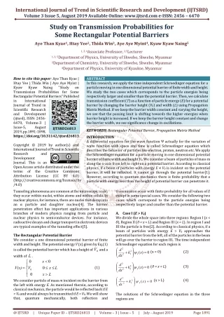
1. International Journal of Trend in Scientific Research and Development (IJTSRD) Volume 3 Issue 5, August 2019 Available Online: www.ijtsrd.com e-ISSN: 2456 – 6470 Study on Transmission Probabilities for Some Rectangular Potential Barriers Aye Than Kyae1, Htay Yee2, Thida Win3, Aye Aye Myint4, Kyaw Kyaw Naing5 1, 3, 4Associate Professor, 2,5Lecturer 1, 3, 5Department of Physics, University of Shwebo, Shwebo, Myanmar 2Department of Chemistry, University of Shwebo, Shwebo, Myanmar 4Department of Physics, University of Kyaukse, Myanmar How to cite this paper: Aye Than Kyae | Htay Yee | Thida Win | Aye Aye Myint | Kyaw Kyaw Naing Transmission Probabilities for Some Rectangular Potential Barriers" Published in International Journal of Trend in Scientific Research and Development (ijtsrd), ISSN: 2456- 6470, Volume-3 | Issue-5, August 2019, pp.1891-1898, https://doi.org/10.31142/ijtsrd26813 Copyright © 2019 by author(s) and International Journal of Trend in Scientific Research and Development Journal. This is an Open Access article distributed under the terms of the Creative Attribution License (http://creativecommons.org/licenses/by /4.0) Tunneling phenomena are common at the microscopic scale; they occur within nuclei, within atoms and within solids. In nuclear physics, for instance, there are nuclei that decay into an α particle and daughter nucleus[4]. The barrier penetration effect has important applications in various branches of modern physics ranging from particle and nuclear physics to semiconductor devices. For instance, radioactive decays and charge transport in electronic devices are typical examples of the tunneling effect[5]. The Rectangular Potential Barrier We consider a one dimensional potential barrier of finite width and height. The potential energy V (x) given by Eq.(1) is called the potential barrier which has a height of width of L .     L L x 0 We consider particle of mass m incident on the barrier from the left with energy E. As mentioned therein, according to classical mechanics, the particle would be reflected back if E < V0and would always be transmitted if E > V0. We will show that, quantum mechanically, ABSTRACT In this research, we apply the time independent Schroedinger equation for a particle moving in one dimensional potential barrier of finite width and height. We study the two cases which corresponds to the particle energies being respectively larger and smaller than the potential barrier. Then, we calculate transmission coefficient (T) as a function of particle energy (E) for a potential barrier by changing the barrier height (V0) and width (L) using Propagation Matrix Method. If we keep the barrier width constant and varying the height, we see that the passing limit is shifting towards the higher energies when barrier height is increased. If we keep the barrier height constant and change the barrier width, we see significance change in oscillations. KEYWORDS: Rectangular Potential Barrier, Propagation Matrix Method INTRODUCTION A differential equation for the wave function Ψ actually for the variation of wave function with space and time is called Schroedinger equation which describes the behavior of particles like electron, proton, neutron etc. We apply the Schroedinger equation for a particle moving in one dimensional potential barrier of finite width and height V0. We consider a beam of particles of mass m along the x-axis from left to right on a potential barrier. According to classical physics, if a beam of particles with energy E < V0 is incident on the potential barrier, it will be reflected. It cannot go through the potential barrier[1]. However, according to quantum mechanics there is finite probability that a particle with energy less than the height of potential barrier can penetrate it. "Study on IJTSRD26813 Commons BY (CC 4.0) transmission occur with finite probability for all values of E except in some special cases. We consider the following two cases which correspond to the particle energies being respectively larger and smaller than the potential barrier. A.Case I (E > V0) We divide the whole space into three regions: Region I (x < 0), Region II (0 < x < L) and Region III (x > L). In region I and III the particle is free[2]. According to classical physics, if a beam of particles with energy E > V0 approaches the potential barrier from the left, all of the particles in the beam will go over the barrier to region III.. The time independent Schroedinger equation for each region is 2     dx 2     dx 2     dx The solutions of the Schroedinger equation in the three regions are V and a   d (x < 0) (2)    0 2 k ( x ) 0 1 1 2  0 x 0     d (0 < x < L) (3)    2 2 k ( x ) 0 (1) V(x) V 0 x 2 2 0     d (x > L) (4)    2 k ( x ) 0 1 3 2 both reflection and @ IJTSRD | Unique Paper ID – IJTSRD26813 | Volume – 3 | Issue – 5 | July - August 2019 Page 1891

2. International Journal of Trend in Scientific Research and Development (IJTSRD) @ www.ijtsrd.com eISSN: 2456-6470 k    2 2         2 mE 2 2 2 ik x ik x k 2 m ( V E ) where potential barrier and propagation directions of the incident, reflected and transmitted waves are shown in Fig.(2) for E < V0. The wave function has an exponential form in the forbidden region inside the barrier. But there is also an oscillator wave to the right of barrier. To find transmission 2 F T  and . The ( x ) A e B e x 0 1 1 1 0 1           ik x ik x (x) ( x ) C e D e 0 x L 2 2 (5) 2      ik x ( x ) F e x L 1 3 k      2 2 2 mE k 2 m ( E V ) coefficients we need only to calculate F in terms where potential barrier and propagation directions of the incident, reflected and transmitted waves are shown in Fig.(1) for E > V0 . The wave function will display an oscillatory pattern in all three regions; its amplitude reduces every time the particle enters a new region. The constants B, C, D and F can be obtained in terms of A from the boundary conditions. The wave functions and their first derivatives must have continuous values[3]. Solving for F, we obtain  2 1 2 1 ( 4   k k e A k k F and . The 1 2 0 2 A of A. The wave functions and their first derivatives must have continuous values. Solving equation for F / A, we obtain    L k e A  1   2 2 k 2 F k k  i k L (10) 1 2 2 cosh ( ) i sinh ( k L )   1 2 2 k 1 2   1  i k L  k i   L k i e L 2 2 ) e ( k k ) 1 2 2 1 2 Fig (2) The potential barrier and the energy E .  1   2 2    2 2 k 2 F k k (11)          2 2 1 T 4 4 cosh ( k L ) sinh ( k L ) 2 2 2     k A 1 2 Fig.1 the potential barrier and the energyE Since   2 2 cosh ( k L ) 1 sinh ( k L ) , we can reduce to    1 2 2     k i L 2 1 2 2 F 4 k k A e 4 k k cos( k L ) 2 i ( k k ) sin( k L ) 1  1 2 1 2 2 2 1   2    2 2 2 k k 1 (6)         2 (12) 1 k T 1 sinh ( k L ) The probability of transmission is given by the transmission coefficient T.     k k A B.Case II (E < V0) According to classical physics, every particle that arrives at the barrier (x = 0) will be reflected back; no particle can penetrate the barrier. However, the quantum mechanical predictions differ sharply from their classical counterparts, for the wave functions is not zero beyond the barrier. In region I (x < 0), and region III (x > L), the Schroedinger equation and its solution remain the same as in case I. In region II (0 < x < L) the Schroedinger equation is 2     dx The solutions of the Schroedinger equation in the three regions are     e F x ) ( 3  2 4 k     1 2 We note that T is finite. This means that the probability for the transmission of the particles into the region is not zero as expected from classical physics. This is a purely quantum mechanical effect which is due to the wave aspect of microscopic objects; it is known as the tunneling effect: quantum mechanical objects can tunnel through classically impenetrable barriers. The Propagation Matrix Method The Propagation Matrix A method is needed a method for finding solutions to complicated potential structures for which analytic expressions are unmanageable. The transmission coefficient is calculated at the first potential step for a particle of energy E incident from the left. We then imagines the transmitted particle propagating to the next potential step, where it again has a probability of being transmitted or reflected. Associated with every potential step and free propagation region to the next potential step is a 2×2 matrix which carries wave function amplitude. The total one dimensional propagation probability for a potential consisting of a number of potential steps may be calculated by multiplying together each 2×2 matrix associated with transmission and reflection at each potential step. Therefore, the wave function coefficients for a particle traversing a one dimensional potential consisting of a number of such regions  1  2 2    F 2 2 2 1 k k  x  0 L    E     2 1 ( 0 V ) T 1 sin ( k L ) (7) 2 2 4     1 2   d  (8)   2 2 k ( x ) 0 2 2      ik x ik x ( x ) A e B e x 0 1 1 1        k x k x (x) ( x ) C e D e 0 x L (9) 2 2 2     ik x x L 1 @ IJTSRD | Unique Paper ID – IJTSRD26813 | Volume – 3 | Issue – 5 | July - August 2019 Page 1892

3. International Journal of Trend in Scientific Research and Development (IJTSRD) @ www.ijtsrd.com eISSN: 2456-6470 may be calculated by multiplying together the appropriate 2×2 matrices. We can solve for a particle moving in an arbitrary potential by dividing the potential into a number of potential energy steps. The following four basic parts are needed. We may use the propagation matrix method to calculate the probability of the electron emerging on the right-hand side of the barrier. The method is best approached by dividing it into small, easy-to-understand, logical parts. The Step Propagation Matrix We calculate the propagation matrix pstep for transmission and reflection of the wave function representing a particle of energy E incident on a single potential step. The potential step we consider is at position xj+1 in Fig.(3). Fig.3 Approximation of a smoothly varying one dimensional potential V(x) with a series of potential steps In this approach, the potential between position xj and xj+1 in region j is approximated by a value Vj. Associated with the potential step at xj and free propagation distance Lj = xj+1 - xj is a 2×2 matrix which carries all of the amplitude and phase information on the particle. Fig.(4) shows detail of the potential step at position index j +1. The coefficients A and C correspond to waves traveling left to right in region j and j +1, respectively. Fig.4 A one dimensional potential step. In region j the potential energy is Vj and in region j+1 the potential energy is Vj+1. The transition between region 1 and region 2 occurs at position x = xj +1. The electron (or particle) has wave vector 2 / 1 )) ( 2 ( j j k  in region j, and the wave functions, which are solutions to the Schrödinger equation in regions j and  m E V  j+1, are   k i x i k x   A e B e j j (13) j j j  i k x i k x    C e D e   j 1 j 1 (14)    j 1 j 1 j 1 Following the convention we have adopted in this paper, A and C are coefficients for the wave function traveling left-to-right in regions j and j+1, respectively, and B and D are the corresponding right-to-left traveling-wave coefficients. The two wave functions given by Eq.(13) and (14) are related to each other by the constraint that ψ and dΨ/dx must be continuous. This means that at the potential step that occurs at the boundary between regions j and j+1 we require @ IJTSRD | Unique Paper ID – IJTSRD26813 | Volume – 3 | Issue – 5 | July - August 2019 Page 1893

4. International Journal of Trend in Scientific Research and Development (IJTSRD) @ www.ijtsrd.com eISSN: 2456-6470    (15)   j j 1 x x   x x j 1  d j 1   d  j j 1  and (16) d x d x   x x x x   j 1 j 1 Substituting Eq.(13) and (14) into Eq.(15) and (16) gives two equations k i j j j e C e B e A 1    k e B e A 1    k i   k i x x x i k x  D k e   j j j 1 j 1 (17)  j 1  k i    i k x i k x k i x x j 1 j 1  C e D e   j j j 1 j 1 (18)  j j j j 1 k k j j By organizing into rows and columns the terms that contain left to right traveling waves of the form eikx and right-to-left traveling waves of the form e−ikx, we may write Eq.(17) and (18) for a potential step at position xj+1= 0 as a matrix equation:       1 1 j j k k We would much prefer a simple equation of the type      1 j j B where pjstep is the 2×2 matrix describing wave propagation at a potential step. To obtain this expression, we need to eliminate the 2×2 matrix on the left-hand side of Eq.(19). We simply use from basic linear algebra that the inverse of a 2×2 matrix    a a   A a a a a A   . Hence, the inverse of   1 1        1 1 2 j j k k where the step matrix is        j j k k  1 1 k     A C   1 1  k  j 1 j (19)           j 1 j 1      B D  j 1 j    A C  j j 1  p (20)     j step D     a a  a a 1 2 a 2 1 2 is where the determinant of A is given by   1 1 1 2 1  A A      a 2 1 1 1 2 1 2 2          1 1 1 1 1 1 is , so that we may write 1 1 1 1 2 2 1 2 2 1         1 1 1 1 2 2  1 1       C C A   1 1 1  (21) k k   j 1 j 1 j   p              j 1 j 1   step D D B   j 1 j 1 j      k k   j 1 j 1 1 1  k k 1   (22) j j p   k k j step 2 1 1   1 1     j j This is our result for the step potential that will be used later. We continue the development of the matrix method by considering the propagation between steps. The Propagation between Steps We calculate the propagation matrix pfree for propagation of the wave function between steps. The free propagation we consider is between positions xj and xj+1 in Fig.(3). The distance of this free propagation is Lj. Propagation between potential  k i L k i L   A e C B e D j j j j steps separated by distance Lj carries phase information only so that expressed in matrix form as        0 e    B    e 0 and . This may be   j j 1 j j 1      C i k L A e 0 k j j  j j 1 (23)         B D i L j j  j j 1    A C  Or, alternatively, (24) j 1 j  P       j free D  j j 1   k i L e 0 j j  p   where (25) j free i k L j j @ IJTSRD | Unique Paper ID – IJTSRD26813 | Volume – 3 | Issue – 5 | July - August 2019 Page 1894

5. International Journal of Trend in Scientific Research and Development (IJTSRD) @ www.ijtsrd.com eISSN: 2456-6470 The Propagation Matrix Pjfor the j-th Region We calculate the propagation matrix for the j-th region in Fig.(3). This is achieved if we multiply pstep and pfree to obtain the propagation matrix Pj for the j-th region of the discretized potential. To find the combined effect of pfree and pjstep we simply multiply the two matrices together. Hence, propagation across the complete j-th element consisting of a free propagation region and a step is    When we multiply out the matrices pjfree pjstep given by Eq.(25) and (22), respectively, it gives us the propagation matrix for the j-th region:           j j j j L k i j L k i j e k k  p p 1 1 1 2   p p p   (26) j jfree jstep p p 2 1 2 2      k k        i k L i k L j 1 j 1    1 e 1 e j j j j k k   1   p p j j p 11 12 = (27)     j     2 * 12 * 11 k k p p           1 1   1 e 1     j j Propagation through an Arbitrary Series of Step Potentials We calculate the total propagation matrix P for the complete potential by multiplying together the propagation matrices for each region of the discretized potential. For the general case of N potential steps, we write down the propagation matrix for each region and multiply out to obtain the total propagation matrix,   j 1 The total propagation matrix Psatisfies continuity in Ψ and dΨ /dx between adjacent regions. Since the particle is introduced from the left, we know that A = 1, and if there is no reflection at the far right then D = 0. We may then rewrite     D D B     0 B In this case, because 1 = p11C, the transmission probability C  j N   (28) P p p . . . p . . . p p 1 2 j N j         A C C j N   j   (29)   p P      j 1   p p    1 C as (30) 1 1 1 2       p p 2 1 2 2 2 is simply 2 (31) 1 2  C p 1 1 Eq.(20) is a particularly simple result. We will make use of this when we calculate the transmission probability of a particle through an essentially arbitrary one-dimensional potential. Transmission Probability for a Rectangular Potential Barrier Fig.(5) is a sketch of the rectangular potential barrier we will consider. The thickness of the barrier is L. A particle of mass m incident from the left of energy E has wave vector k1. In the barrier region, the wave vector is k2. The wave vector k1 and k2 are related through 0 2 1 / 2  V m k k   . 2 2 2 Fig.5 The potential of a one dimensional rectangular barrier of energy V0 @ IJTSRD | Unique Paper ID – IJTSRD26813 | Volume – 3 | Issue – 5 | July - August 2019 Page 1895

6. International Journal of Trend in Scientific Research and Development (IJTSRD) @ www.ijtsrd.com eISSN: 2456-6470  x 0 A wavy particle incident on the barrier from the left with amplitude A sees a potential step-up in energy of barrier propagation region of length L , and a potential step-down at 1k outside the barrier and change in potential between two regions in which the wave vector changes from k1 to k2 due to the potential step up shown in Fig.(3). The corresponding wave function changes from ψ1 to ψ2. Solutions of the Schroedinger equation for a step change in potential are B e k 1 1 D e k 2 2 V at , a 0 x  0 L x  . A particle of energy E , mass m , and charge e L . We consider a particle impinging on a step  2 k in the barrier region has wave number A  i k x i k x   1 1 Ψ e (32) 1 k C  i k x i k x   2 2 Ψ e (33) 2 k  Ψ Ψ Applying the condition that the wave function is continuous at the potential step and that the derivative 1 2 step step dΨ dΨ  of the wave function is continuous gives 1 2 dx dx step step A B C D    (34) k A k B k k k 1 1 2 2 k C D    2 2 (35) k k k k k k 1 1 1 1 2 2 Rewritten in matrix form, these equations become    k B k 2 1 1 1 To eliminate the 2 × 2 matrix on the left-hand side of this equation, we must find and multiply by its inverse matrix. The 2 ) 1 1 ( k k     , so the inverse of the left-hand matrix is   1 1      1 1 A C 1 1   k k (36)        2 2     D k k 1 1   1 1 k determinant of the left-hand matrix is . Hence, 1   1 1  1 1 2 k 1 we may rewrite Eq. (36) as   1 1             k k A 1 1 C 1 1 C k 2 1 1 1  k k  1 1   1              2 2        k k B 1 1 D 1 1 D k k 2 k k k k 2 2 1 2 1 2 1 1 Multiplying out the two square matrices gives the   k k k B 1 2 1 2 Since the rectangular potential barrier consists of a step up and a step down, we can make use of this symmetry and immediately calculate the 2 × 2 matrix for the step down by simply interchanging k1 and k2. The total propagation matrix for the rectangular potential barrier of thickness L consists of the step-up 2 × 2 matrix multiplied by the propagation matrix from the barrier thickness L multiplied by the step-down matrix. Hence, our propagation matrix become    2 1 2 1 2 1 2 0 2 e k k k k k k       2 2 1 2 1 2 1 ) ( ) ( 4 k e k k e k k k k To find the matrix elements of P, we just multiply out the matrices in Eq.(38). For example k k p    (39) 2 2 matrix describing propagation at the step-up in potential        k k k k A C 1 1 2 1 2  (37)        k k k D 2 1 2           i k L k k k k k k k k e 0 1 1 k 2 1 2 1 2 2 1 2 1  P           i k L k k k k k 2 2 1 2 1 1 2         i k L i k L k k k k ( k k ) e ( k k ) e 1 2 2 2 1 2 1  1 2 1 2 P    (38)    i k L i k L k k k 2 2 1 2 1 p becomes 12  2 2 2 k i  k i L L 1 ( e e ) 2 2 12 4 k k 1 2 @ IJTSRD | Unique Paper ID – IJTSRD26813 | Volume – 3 | Issue – 5 | July - August 2019 Page 1896

7. International Journal of Trend in Scientific Research and Development (IJTSRD) @ www.ijtsrd.com eISSN: 2456-6470 The next step we want to take is to calculate the transmission probability for a particle incident on the barrier. We already 2 1 know that the transmission of a particle incident from the left is given by , so that we will be interested in p 1 1 p from Eq.(38) )( k k  obtaining 11 i k L k i      L ( k k ) e ( k k )( k k ) e 2 2  2 1 1 2 1 2 2 1 p (40) 11 4 k k  1 2 ( k ) k i      L k i L 2 2 2 2 2 2 ( k k 2 k k ) e k k 2 k k ) e 2 2  1 1 2 1 1 2 p (41) 11 4 k 1 2 k i  k i     L k i L L i k L 2 2 2 ( k k )( e e 2 k k ( e e ) 2 2 2 2   1 1 2 p (42) 11 4  k k k ( ) 4 k k 1 2 1 2 k i   k i L L 2 2 2 ( k e e ) 1 1 2 2      i k L k i L 1 p ( e e ) 2 2 (43) 11 2 1 2 ( ) k k 2 1 1 e 2 k i    k i L L 2 2 2 ( k k e ) 2 2      i k L k i L 1 p ( e e ) 2 2 (44) 11 2 2 k k 2 1 2 The Result and Discussion We use the propagation matrix approach to calculate the transmission coefficient T of a rectangular potential barrier with width L = 1nm and height V0= 0.3 eV as shown in Fig.(5). Matrix technique in transmission calculations means that we express every region of barrier as a propagation matrix P. The transmission coefficient can be expressed 1 T  . Using this principle, transmission coefficient T 2 p 1 1 dependence on electron energy for a rectangular potential barrier was numerically calculated in Fig.(6). We vary barrier width while keeping barrier height constant. Transmission probabilities T (E) for barrier height V0 = 0.3 eV and width L = 0.2 nm to 3.2 nm by increasing twice of initial value are shown in Fig.(7) to Fig.(11) respectively. Fig.(12) shows the transmission probability T (E) for barrier height V0 = 0.3 eV and different barrier width. Fig.(7) Numerical calculation of transmission coefficient for a barrier of height V0 = 0.3 eV and width L = 0.2 nm. Fig.(6) The transmission coefficient T for a barrier of width L = 1 nm and height V0 = 0.3 eV. Fig.(8) Numerical calculation of transmission coefficient for a barrier of height V0 = 0.3 eV and width L = 0.4 nm. @ IJTSRD | Unique Paper ID – IJTSRD26813 | Volume – 3 | Issue – 5 | July - August 2019 Page 1897

8. International Journal of Trend in Scientific Research and Development (IJTSRD) @ www.ijtsrd.com eISSN: 2456-6470 Fig.(9) Numerical calculation of transmission coefficient for a barrier of height V0 = 0.3 eV and width L = 0.8 nm. Fig.(12) Numerical calculation of transmission coefficient for a barrier of height V0 = 0.3 eV and different width. When a beam of particles of fixed energy is incident on a potential barrier, a certain fraction of the incident particles is transmitted while the remaining fraction is reflected. This is in contrast to classical mechanics. Classically, there must be total transmission if the energy of the incident particle is more than the height of the barrier, and total reflection if the energy of the incident particle is less than the height of the barrier. Fig.(12) shows the transmission probability T(E) for barrier height V0 = 0.3 eV and different barrier width. If we keep the barrier height constant and change the barrier width, we see significance change in oscillations. When barrier width is narrow, even electron with lower energy can pass through the barrier by quantum tunneling. The wider the barrier will be the less observable the tunneling is, which is expectation from classical approach as well. Conclusion We have found that the transmission coefficient (T) depends upon potential barrier height (V0) and barrier width (L). The transmission coefficient (T) is a measure of the probability that the particle will be transmitted through the barrier. Thus, we conclude that there is finite probability of particle penetrating the barrier and appearing on the other sides. The ability of particle to penetrate the barrier when E < V0is a quantum mechanical result and is known as tunnel effect. In nuclear physics, there are nuclei that decay into an α particle and daughter nucleus. This α decay process can be explained by tunnel effect. ACKNOWLEDGEMENTS We thank all the people for their help directly and indirectly to complete our study. REFERENCES [1]G. S. CHADDHA, “Quantum Mechanics”, New Age International (P) Ltd, Publishers, New Delhi, (2003). [2]R. Murugeshan, “Modern Physics”, S. Chand & Company Ltd, India, (1997). [3]M. C. Jain, Quantum Mechanics, “A Textbook for Undergraduates”, Prentice-Hall of India Private Ltd, New Delhi, (2007). [4]N. Zettili, “Quantum Mechanics”, John Wiley & Sons, Ltd, England, (2001). [5]A. F. J. Levi, “Applied Quantum Mechanics”, Cambridge University Press,(2006). Fig.(10) Numerical calculation of transmission coefficient for a barrier of height V0 = 0.3 eV and width L = 1.6 nm. Fig.(11 ) Numerical calculation of transmission coefficient for a barrier of height V0 = 0.3 eV and width L = 3.2 nm. @ IJTSRD | Unique Paper ID – IJTSRD26813 | Volume – 3 | Issue – 5 | July - August 2019 Page 1898