Download
1 / 3
30 likes | 45 Vues
The year 2020 has indeed experienced a shaking pandemic of the modern age. While all the concerned departments all over the world are religiously doing their duties to contain the spread of the infection, it was thought of to put forward a paper on the understanding of various graphs presented by the authorities from time to time which indicate the total number of cases, number of active cases, number of recoveries and number of deaths. This paper deals with the understanding of two main types of plots i.e. linear and logarithmic and shall highlight details of various functions and their trends. A phrase, Flattening the curve has been in use these days. This paper shall first build a premise and then explain the qualitative meaning of the phrase in the context of the plots. Various psychological aspects shall also be appended so that the reader can be benefitted and can be made ready to understand the current affairs. Gourav Vivek Kulkarni "Qualitative Understanding of Flattening the Curve Term in Context of COVID-19" Published in International Journal of Trend in Scientific Research and Development (ijtsrd), ISSN: 2456-6470, Volume-4 | Issue-4 , June 2020, URL: https://www.ijtsrd.com/papers/ijtsrd30926.pdf Paper Url :https://www.ijtsrd.com/mathemetics/statistics/30926/qualitative-understanding-of-flattening-the-curve-term-in-context-of-covid19/gourav-vivek-kulkarni<br>

E N D
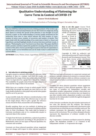
International Journal of Trend in Scientific Research and Development (IJTSRD) Volume 4 Issue 4, June 2020 Available Online: www.ijtsrd.com e-ISSN: 2456 – 6470 Qualitative Understanding of Flattening the Curve Term in Context of COVID-19 Gourav Vivek Kulkarni B.E. Mechanical, KLS Gogte Institute of Technology, Belagavi, Karnataka, India ABSTRACT The year 2020 has indeed experienced a shaking pandemic of the modern age. While all the concerned departments all over the world are religiously doing their duties to contain the spread of the infection, it was thought of to put forward a paper on the understanding of various graphs presented by the authorities from time to time which indicate the total number of cases, number of active cases, number of recoveries and number of deaths. This paper deals with the understanding of two main types of plots i.e. linear and logarithmic and shall highlight details of various functions and their trends. A phrase, "Flattening the curve" has been in use these days. This paper shall first build a premise and then explain the qualitative meaning of the phrase in the context of the plots. Various psychological aspects shall also be appended so that the reader can be benefitted and can be made ready to understand the current affairs. KEYWORDS: Curve, Flatten, Linear, Logarithmic, Cumulative, COVID-19 How to cite this paper: Gourav Vivek Kulkarni "Qualitative Understanding of Flattening the Curve Term in Context of COVID-19" Published in International Journal of Trend in Scientific Research and Development (ijtsrd), ISSN: 2456- 6470, Volume-4 | Issue-4, June 2020, pp.228-230, www.ijtsrd.com/papers/ijtsrd30926.pdf Copyright © 2020 by author(s) and International Journal of Trend in Scientific Research and Development Journal. This is an Open Access article distributed under the terms of the Creative Commons Attribution License (CC (http://creativecommons.org/licenses/by /4.0) IJTSRD30926 URL: BY 4.0) A.Introduction to plotting graphs A graph is meant to concisely and precisely represent a large quantum of data in a manner such that the reader can comprehend the range of data, key points and overall trend. Thus it is imperative for a graph that it should be readable. The readability of a graph comes from the right selection of scale and the range of data to be included. While there are a number of ways in which graphs can be plotted like line graph, bar graph, pie chart and so on, this study shall be limited to a line graph only and all other graphs shall be out of its purview. In any scientific study, the reference considered plays a vital role in interpretation of data. The reference may or may not be the origin always. Thus to plot a graph, the reference chosen should be fixed, measurable and unambiguous. Broadly speaking, there are two methods of plotting two dimensional line graphs viz. in Cartesian Coordinates and the other in Polar Coordinates. This study shall be limited to Cartesian coordinates only as it is considerably simpler to represent data in this manner. To begin from the basics, by definition, a physical quantity is one that can be measured. According to the perspective of Mathematics, there are two types of Physical Quantities viz. constants and variables. Constants are those physical quantities whose magnitude does not change with respect to other physical quantities. There are two types of constants viz. numerical constant and arbitrary constant. A numerical constant is a constant whose numerical value is known while an arbitrary constant is one whose numerical value is not known but it is known that it is a constant. Variables are those physical quantities whose magnitude varies with respect to other physical quantities. There are two types of variables viz. independent variable and dependent variable. Independent variable is that which can assume any value and whose variation does not depend on any other variable while a dependent variable is one which depends on the independent variable through the designated function for its value. In the Cartesian coordinates, the plot includes intersection of two axes; the abscissa and the ordinate. The abscissa represents the independent variable and is also known as the horizontal axis on which the process variables can be set. The ordinate represents the dependent variable and is also known as the vertical axis. The curve thus obtained in the plot represents the dependence of ordinate variable on the abscissa variable. Fig. 1 represents a Cartesian coordinate system for plotting graphs. The dependent variable 'y' is a function of the independent variable 'x'. 0 represents the origin @ IJTSRD | Unique Paper ID – IJTSRD30926 | Volume – 4 | Issue – 4 | May-June 2020 Page 228
International Journal of Trend in Scientific Research and Development (IJTSRD) @ www.ijtsrd.com eISSN: 2456-6470 The logarithmic scale starts from unity as logarithm of 0 is undefined. From the figure it can be observed that the abscissa is represented by a linear scale while the ordinate is represented by a logarithmic scale. On the logarithmic scale, the abscissa represents the common logarithm of unity. Every succeeding line is offset at a distance equal to the corresponding common logarithm. By this, the line representing 10 is at 1 unit linear distance from the abscissa, that representing 100 is at 2 units distance, 1000 is at 3 units distance and so on. The intermediate points are at corresponding logarithmic distance. Thus a considerable large range of values can be represented using a logarithmic scale which would otherwise not be possible that easily in case of a linear scale. Fig.1: Cartesian Coordinate system for plotting graphs For the given experiment, values of the dependent variable 'x' can be set and the corresponding values of y obeying the function y = f(x) can be plot on the graph as per the range and scale. Range in a graph covers all the values of the independent and dependent variables while the scale ensures that all these values fit in the given area so that the readability of the graph is maintained throughout. Thus for a finite range of values on the abscissa, a much larger range of values can be represented on the ordinate by employing the logarithmic scale. D.Various COVID-19 statistical plots and desired trends With the aspects discussed till now, the subject of various plots related to COVID-19 shall be taken up. Medical aspects shall be out of purview of this paper and the statistical aspects related to plotting of graphs shall be in the purview. Next two sections shall highlight two scales in which graphs can be drawn in order to represent data. B.Plotting on a linear scale As the name itself indicates, a linear scale refers to equal sub divisions of intervals in a graph on both the axes. The ratio of values on the axes may or may not be equal to unity but the division definitely follows a linear increase or decrease in values to be plot. Linear scale is employed for whole numbers as well as natural numbers. There are four plots that form the basis of statistical study of COVID-19 viz. No. of Confirmed cases, No. of Active cases, No. of Recoveries and No. of Deaths. Each of these shall be discussed as follows. Linear scale is used when the range of values is small and the variations of dependent variable with respect to independent variable are not exponential in nature. This implies that for higher powers of the abscissa, depending on the function, it may be required that the scale on the ordinate accommodates the higher values as well. This itself paves way to plotting on a logarithmic scale which is discussed as follows. In all the plots, the abscissa shall represent the number of days in linear scale and the ordinate shall represent the said variable in terms of cumulative No. of cases in different categories in logarithmic scale. Logarithmic scale is recommended considering the previous experience of exponential increase in cumulative number of cases due to the outbreak of such similar pandemics. D.1. Plot of No. of Confirmed Cases v/s Days This plot represents the cumulative number of cases confirmed in a sample space. The sample space may be a district, a state or the nation itself. C.Plotting on a logarithmic scale As indicated in the previous section, the logarithmic scale is typically used when there is sudden variation in the magnitude of the ordinate over a considerably small range of the abscissa. These graphs are useful to represent exponential trends. Logarithmic scale is employed for natural numbers as natural or common logarithm of 0 is undefined. This is an independent curve which gets its values as a result of testing carried out for infection. With every passing day, the number of newly confirmed cases is added to the existing sum. This cumulative number of cases is plot on the logarithmic scale of the ordinate. Generally, the abscissa is kept linear but there are certain graphs wherein the abscissa and ordinate are fixed in logarithmic scale. It is natural that with every passing day, until an effective vaccine is prepared, new cases are confirmed if necessary precautions are not taken. The motive of monitoring this curve would be that the least possible number of cases are confirmed everyday in order to proclaim that the pandemic is under control. In the linear scale, every successive point is equidistant from the previous point but in a logarithmic scale, every point is at a logarithmic distance from its preceding point. Fig. 2 represents the logarithmic plot with linear scale on abscissa An increasing curve indicates increase in the number of cases for each passing day while a decreasing curve is not feasible in this plot. A curve parallel to the abscissa represents no increase in the number of cases and hence proclaims the control over the pandemic in the considered sample space. Thus the desired trend of this plot would be a curve parallel to the abscissa with each passing day which is a flat curve. D.2. Plot of No. of Active Cases v/s Days This plot represents the cumulative number of cases active in a sample space as considered while plotting the cumulative Fig. 2: Logarithmic scale on ordinate and linear scale on abscissa @ IJTSRD | Unique Paper ID – IJTSRD30926 | Volume – 4 | Issue – 4 | May-June 2020 Page 229
International Journal of Trend in Scientific Research and Development (IJTSRD) @ www.ijtsrd.com eISSN: 2456-6470 number of confirmed cases. It is the difference between number of confirmed cases and the sum of number of recovered cases and number of deaths. Thus the desired trend of this plot would be a curve parallel to the abscissa with each passing day which is a flat curve. E.Qualitative understanding of the term - Flattening the curve Except the curve representing the cumulative number of active cases, the desired trend for all the other three curves is a line parallel to the abscissa representing a flat curve. This is the most dependent curve among all the four. With every passing day, there may be increase or decrease in the number of confirmed cases based on the degree of effective measures been implemented to curb the infection, also depending on the medical facilities, medicines, treatments and response from the patients, the number of recoveries and deaths will b reported. Thus the curve of cumulative number of active cases may not show stability as a certain trend. It is here itself that the term flattening the curve comes into picture. Theoretically, it may seem easy to extrapolate and predict the trends of the curves but it is the actual data that enables the success of the prediction. On a given day, if the number of confirmed cases are 100, number of recoveries are 90 and deaths are 0, the number of active cases becomes 10. On the next day, if 50 more cases are confirmed with 45 recoveries and 0 deaths, the cumulative number of confirmed cases now becomes 150 while the number of cumulative number of recoveries becomes 135 thus leading to 15 active cases at the end of two days. It can be observed that although the percentage of recovery per day is same i.e. 90%, the number of active cases varies. This itself makes the plot of cumulative number of active cases quite unstable and dependent on various variables over a period of many days. Flattening the curve thus means control over various variables to prevent outbreak through community transfer and mutual infection in order to gradually reduce the number of confirmed cases day by day so that the curve assumes a trend to become flat on the logarithmic scale. This gives apt understanding of the term flattening of the curve. In case of number of confirmed cases, this can be achieved when lesser and lesser number of cases are reported everyday so that the change in cumulative number of cases is meager and the curve is almost flat. In case of number of recoveries, if the number of confirmed cases is a flat curve, with adequate treatment and reciprocal response from the infected patient, the curve can be flattened automatically In case of number of deaths, if care is taken right from the beginning, the number of cumulative deaths with each passing day with automatically represent a flat curve. This is the only curve which can exhibit a negative trend for the cumulative values. This is possible when the sum of number of recoveries and deaths exceeds the number of reported cases. In such case, the number of active cases becomes negative. Thus the desired trend of this plot would be a decreasing curve with each passing day which tends to the abscissa. F.Psychological aspects of reading the curves In the contemporary world, although we may not be experts in the fields of medical science, virology, statistics or any such specializations, there is an inquisitive sense of eagerness to know the current situation which makes us follow the news and read the graphs represented. This paper is intended to provide basic aid to read the same. D.3. Plot of No. of Recoveries v/s Days This plot represents the cumulative number of recovered cases as of a given day in the sample space. This plot is independent of the number of cases reported in a day or the number of deaths as number of recoveries and number of deaths are the only two possible outcomes. Thus according to Probability theory, since every random experiment has an outcome and depending on the evaluator, the same may be desirable or undesirable, either the patient may be discharged post recovery or may pass away. Graphs based on daily records have not been considered in this paper to avoid confusion. In addition to this, flattening the curve is possible only in case of data that is represented in a cumulative manner and daily records are never reported in cumulative manner. With every passing day, depending on the medical variables, certain number of patients get cured and are discharged. This is added to the cumulative number and is plotted on a graph that indicates the number of recoveries. Psychological well being is a personal issue. There are optimistic views, pessimistic views, practical views and impractical views as well. However this study is intended to provide basic knowledge of the curves and the methodology to read the same so that one can stay updated with high morale for a better future. Since the term flattening the curve needs to be understood well and monitored, this paper can be considered as an effort to create awareness. Ideally, this graph should always have an increasing trend but if there are lesser and lesser active cases with every passing day, this graph with tend to be parallel to the abscissa. Thus the desired trend of this plot would be a curve that is initially increasing and then parallel to the abscissa with each passing day which is a flat curve. Conclusion Thus it can be concluded that the term flattening the curve has been qualitatively defined with explanation of linear and logarithmic scales of plotting graphs that represent plots of various types of data v/s number of days like cumulative number of confirmed cases, cumulative number of active cases, cumulative number of recoveries and cumulative number of deaths. Towards the end certain psychological aspects have been considered related to the awareness required with respect to such pandemics. D.4. Plot of No. of Deaths v/s Days This plot represents the cumulative number of deaths as of a given day in the sample space. This is the second probable outcome of the infection. This curve is also an independent curve. Ideally, it is expected that this curve never exhibits an increasing trend but it may happen that due to lack of infrastructure or lack of adequate immunity in the patient itself, there may be variation in the number of deaths with each passing day. @ IJTSRD | Unique Paper ID – IJTSRD30926 | Volume – 4 | Issue – 4 | May-June 2020 Page 230