Transient Thermal Response
Transient Thermal Response. Transient Models Lumped: Tenbroek (1997), Rinaldi (2001), Lin (2004) Introduce C TH usually with approximate Green’s functions; heated volume is a function of time (Joy, 1970) Finite-Element methods. Instantaneous T rise.

Transient Thermal Response
E N D
Presentation Transcript
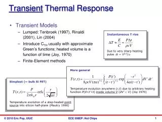
Transient Thermal Response • Transient Models • Lumped: Tenbroek (1997), Rinaldi (2001), Lin (2004) • Introduce CTH usually with approximate Green’s functions; heated volume is a function of time (Joy, 1970) • Finite-Element methods Instantaneous T rise Due to very sharp heating pulse t ‹‹ V2/3/ More general Simplest (~ bulk Si FET) Temperature evolution anywhere (r,t) due to arbitrary heating function P(0<t’<t) inside volume V (dV’ V) (Joy 1970) Temperature evolution of a step-heated point source into silicon half-plane (Mautry 1990)
Instantaneous Temperature Rise • Neglect convection & radiation • Assuming lumped body • Biot = hL/k << 1, internal resistance and T variation neglected, T(x) = T = const. L Instantaneous T rise d W Due to very sharp heating pulse t ‹‹ V2/3/
Lumped Temperature Decay • After power input switched off • Assuming lumped body • RTH = 1/hA • CTH = cV • Time constant ~ RTHCTH L T decay d W T(t=0) = TH
Electrical and Mechanical Analogy • Thermal capacitance (C = ρcV) normally spread over the volume of the body • When Biot << 1 we can lump capacitance into a single “circuit element” (electrical or mechanical analogy) There are no physical elements analogous to mass or inductance in thermal systems
Transient Edge (Face) Heating When is only the surface of a body heated? I.e. when is the depth dimension “infinite”? Note: Only heated surface B.C. is available Lienhard book, http://web.mit.edu/lienhard/www/ahtt.html Also http://www.uh.edu/engines/epi1384.htm
Transient Heating with Convective B.C. • If body is “semi-infinite” there is no length scale on which to build the Biot number • Replace Biot (αt)1/2 Note this reduces to previous slide’s simpler expression (erf only) when h=0!
Transient Lumped Spreading Resistance Source: TimoVeijola, http://www.aplac.hut.fi/publications/bec-1996-01/bec/bec.html • Point source of heat in material with k, c and α = k/c • Or spherical heat source, outside sphere • This is OK if we want to roughly approximate transistor as a sphere embedded in material with k, c ~ Bulk Si FET transient Temperature evolution of a step-heated point source into silicon half-plane (Mautry 1990) Characteristic diffusion length LD = (αt)1/2
Transient of a Step-Heated Transistor In general: “Instantaneously” means short pulse time vs. Si diffusion time (t < LD2/α) or short depth vs. Si diffusion length (L < (αt)1/2) Carslaw and Jaeger (2e, 1986)
Temperature of Pulsed Diode Holway, TED 27, 433 (1980)
Transient of a Step-Heated Interconnect When to use “adiabatic approximation” and when to worry about heat dissipation into surrounding oxide
Understanding the sqrt(t) Dependence • Physical = think of the heated volume as it expands ~ (αt)1/2 • Mathematical = erf approximation
Time Scales of Thermal Device Failure • Three time scales: • “Small” failure times: all heat dissipated within defect, little heat lost to surrounding ~ adiabatic (ΔT ~ Pt) • Intermediate time: heating up surrounding layer of (αt)1/2 • “Long” failure time ~ steady-state, thermal equilibrium established: ΔT ~ P*const. = PRTH
Ex: Failure of SiGe HBT and Cu IC Wunsch-Bell curve of HBT
Ex: Failure of Al/Cu Interconnects Banerjee et al., IRPS 2000 • Fracture due to the expansion of critical volume of molten Al/Cu. (@ 1000 0C) Ju & Goodson, Elec. Dev. Lett.18, 512 (1997)
Temperature Rise in Vias S. Im, K. Banerjee, and K. E. Goodson, IRPS 2002 Via and interconnect dimensions are not consistent from a heat generation / thermal resistance perspective, leading to hotspots. New model accounts for via conduction and Joule heating and recommends dimensions considering temperature and EM lifetime. Based on ITRS global lines of a 100 nm technology node (Left: ANSYS simulation. Right: Closed-Form Modeling)
Time Scales of Electrothermal Processes Source: K. Goodson
ESD: Electrostatic Discharge J. Vinson & J. Liou, Proc. IEEE 86, 2 (1998) • High-field damage • High-current damage • Thermal runaway … …
Common ESD Models Gate J. Vinson & J. Liou, Proc. IEEE 86, 2 (1998) Source Drain Combined, transient, electro-thermal device models Lumped: Human-Body Model (HBM) Lumped: Machine Model (MM)
Reliability Source: M. Stan Ea = 1.1 eV • The Arrhenius Equation: MTF=A*exp(Ea/kBT) • MTF: mean time to failure at T • A: empirical constant • Ea: activation energy • kB: Boltzmann’s constant • T: absolute temperature • Failure mechanisms: • Die metalization (Corrosion, Electromigration, Contact spiking) • Oxide (charge trapping, gate oxide breakdown, hot electrons) • Device (ionic contamination, second breakdown, surface-charge) • Die attach (fracture, thermal breakdown, adhesion fatigue) • Interconnect (wirebond failure, flip-chip joint failure) • Package (cracking, whisker and dendritic growth, lid seal failure) • Most of the above increase with T (Arrhenius) • Notable exception: hot electrons are worse at low temperatures Ea = 0.7 eV
Improved Reliability Analysis M. Stan (2007), Van der Bosch, IEDM (2006) • There is NO “one size fits all” reliability estimate approach • Typical reliability lifetime estimates done at worst-case temperature (e.g. 125 oC) which is an OVERDESIGN • Apply in a “lumped” fashion at the granularity of microarchitecture units life consumption rate
Combined Package Model Steady-state: Tj – junction temperature Tc – case temperature Ts – heat sink temperature Ta – ambient temperature
Thermal Design Summary • Temperature affects performance, power, and reliability • Architecture-level: conduction only • Very crude approximation of convection as equivalent resistance • Convection, in general: too complicated, need CFD! • Use compact models for package • Power density is key • Temporal, spatial variation are key • Hot spots drive thermal design