Download
1 / 24
240 likes | 266 Vues
MA/CSSE 474 Theory of Computation. Bottom-up parsing Pumping Theorem for CFLs. Recap: Going One Way. Lemma : Each context-free language is accepted by some PDA. Proof (by construction): The idea: Let the stack do the work. Two approaches: Top down Bottom up. Example from Yesterday.

E N D
MA/CSSE 474 Theory of Computation Bottom-up parsingPumping Theorem for CFLs
Recap: Going One Way Lemma: Each context-free language is accepted by some PDA. Proof (by construction): The idea: Let the stack do the work. Two approaches: • Top down • Bottom up
Example from Yesterday L = {anbmcpdq : m + n = p + q} 0 (p, , ), (q, S) (1) SaSd 1 (q, , S), (q, aSd) (2) ST 2 (q, , S), (q, T) (3) SU 3 (q, , S), (q, U) (4) TaTc 4 (q, , T), (q, aTc) (5) TV 5 (q, , T), (q, V) (6) U bUd 6 (q, , U), (q, bUd) (7) UV 7 (q, , U), (q, V) (8) VbVc 8 (q, , V), (q, bVc) (9) V 9 (q, , V), (q, ) 10 (q, a, a), (q, ) 11 (q, b, b), (q, ) input = a a b c c d 12 (q, c, c), (q, ) 13 (q, d, d), (q, ) trans state unread input stack
The Other Way to Build a PDA - Directly L = {anbmcpdq : m + n = p + q} (1) SaSd (6) UbUd (2) ST (7) UV (3) SU (8) VbVc (4) TaTc (9) V (5) TV input = a a b c d d a//a b//a c/a/ d/a/ b//a c/a/ d/a/ 1 2 3 4 c/a/ d/a/ d/a/
Notice the Nondeterminism Machines constructed with the algorithm are often nondeterministic, even when they needn't be. This happens even with trivial languages. Example: AnBn = {anbn: n 0} A grammar for AnBn is: A PDA M for AnBn is: (0) ((p, , ), (q, S)) [1] SaSb (1) ((q, , S), (q, aSb)) [2] S (2) ((q, , S), (q, )) (3) ((q, a, a), (q, )) (4) ((q, b, b), (q, )) But transitions 1 and 2 make M nondeterministic. A directly constructed machine for AnBn can be deterministic. Constructing deterministic top-down parsers major topic in CSSE 404.
Bottom-Up PDA The idea: Let the stack keep track of what has been found. Discover a rightmost derivation in reverse order. Start with the sentence and try to "pull it back" (reduce) to S. (1) EE + T (2) ET (3) TTF (4) TF (5) F (E) (6) Fid Reduce Transitions: (1) (p, , T + E), (p, E) (2) (p, , T), (p, E) (3) (p, , FT), (p, T) (4) (p, , F), (p, T) (5) (p, , )E( ), (p, F) (6) (p, , id), (p, F) Shift Transitions: (7) (p, id, ), (p, id) (8) (p, (, ), (p, () (9) (p, ), ), (p, )) (10) (p, +, ), (p, +) (11) (p, , ), (p, ) Parse the string:id + id * id When the right side of a production is on the top of the stack, we can replace it by the left side of that production… …or not! That's where the nondeterminism comes in: choice between shift and reduce; choice between two reductions.
A Bottom-Up Parser The outline of M is: M = ({p, q}, , V, , p, {q}), where contains: ● The shift transitions: ((p, c, ), (p, c)), for each c. ● The reduce transitions: ((p, , (s1s2…sn.)R), (p, X)), for each rule Xs1s2…sn. in G. Undoes an application of this rule. ● The finish-up transition: ((p, , S), (q, )). Top-down parser discovers a leftmost derivation of the input string (If any). Bottom-up parser discovers a rightmost derivation (in reverse order)
Acceptance by PDA derived from CFG • Much more complex than the other direction. • Nonterminals in the grammar we build from the PDA M are based on a combination of M's states and stack symbols. • It gets very messy. • Takes 10 dense pages in the textbook. • I think we can use our limited course time better.
How Many Context-Free Languages Are There? (we had a slide just like this for regular languages) Theorem:There is a countably infinite number of CFLs. Proof: ● Upper bound: we can lexicographically enumerate all the CFGs. ● Lower bound: {a}, {aa}, {aaa}, … are all CFLs. The number of languages is uncountable. Thus there are more languages than there are context-free languages. So there must be some languages that are not context-free.
Languages That Are and Are Not Context-Free a*b* is regular. AnBn = {anbn : n 0} is context-free but not regular. AnBnCn = {anbncn : n 0} is not context-free. Is every regular language also context-free?
Showing that L is Context-Free Techniques for showing that a language L is context-free: 1. Exhibit a context-free grammar for L. 2. Exhibit a PDA for L. 3. Use the closure properties of context-free languages. Unfortunately, these are weaker than they are for regular languages. union,reverse, concatenation, Kleene star intersection of CFL with a regular language NOT intersection, complement, set difference
Showing that L is Not Context-Free Recall the basis for the pumping theorem for regular languages: A DFSM M. If a string is longer than the number of M's states… Why would it be hard to use a PDA to show that long strings from a CFL can be pumped?
Some Tree Geometry Basics The height h of a tree is the length of the longest path from the root to any leaf. The branching factor b of a tree is the largest number of children associated with any node in the tree. Theorem: The length of the yield (concatenation of leaf nodes) of any tree T with height h and branching factor b is bh. Done in CSSE 230.
A Review of Parse Trees A parse tree, (a.k.a. derivation tree) derived from a grammar G = (V, , R, S), is a rooted, ordered tree in which: ● Every leaf node is labeled with an element of {}, ● The root node is labeled S, ● Every interior node is labeled with an element of N(i.e., V - ), ● If m is a non-leaf node labeled X and the children of m (left-to-right on the tree) are labeled x1, x2, …, xn, then the rule X x1x2 … xn is in R.
From Grammars to Trees Given a context-free grammar G: ● Let n be the number of nonterminal symbols in G. ● Let b be the branching factor of G Suppose that a tree T is generated by G and no nonterminal appears more than once on any path: The maximum height of T is: The maximum length of T’s yield is:
The Context-Free Pumping Theorem We use parse trees, not machines, as the basis for our argument. Let L = L(G), and let wL. Let T be a parse tree for w such that has the smallest possible number of nodes among all trees based on a derivation of w from G. Suppose L(G) contains a string w such that |w| is greater than bn. Then its parse tree must look like (for some nonterminal X): X[1] is the lowest place in the tree for which this happens. I.e., there is no other X in the derivation of x from X[2].
The Context-Free Pumping Theorem There is another derivation in G: S* uXz* uxz, in which, at X[1], the nonrecursive rule that leads to x is used instead of the recursive one that leads to vXy. So uxz is also in L(G). Derivation of w
The Context-Free Pumping Theorem There are infinitely many derivations in G, such as: S* uXz* uvXyz * uvvXyyz* uvvxyyz Those derivations produce the strings: uv2xy2z, uv3xy3z, uv4xy4z, … So all of those strings are also in L(G).
The Context-Free Pumping Theorem If rule1 is XXa, we could have v = . If rule1 is XaX, we could have y = . But it is not possible that bothv and y are . If they were, then the derivation S* uXz* uxz would also yield w and it would create a parse tree with fewer nodes. But that contradicts the assumption that we started with a parse tree for w with the smallest possible number of nodes.
The Context-Free Pumping Theorem The height of the subtree rooted at [1] is at most: So |vxy| .
The Context-Free Pumping Theorem If L is a context-free language, then k 1 ( strings wL, where |w| k (u, v, x, y, z ( w = uvxyz, vy, |vxy| k, and q 0 (uvqxyqz is in L)))). Write it in contrapositive form. Try to do this before going on.
Pumping Theorem contrapositive • We want to write it in contrapositive form, so we can use it to show a language is NOT context-free. Original: If L is a context-free language, then k 1 ( strings wL, where |w| k (u, v, x, y, z (w = uvxyz, vy, |vxy| k, and q 0 (uvqxyqz is in L)))). Contrapositive: If k 1 ( string wL, where |w| k (u, v, x, y, z (w = uvxyz, vy, |vxy| k, and q 0 (uvqxyqz is not in L)))), then L is not a CFL.
Regular vs. CF Pumping Theorems Similarities: ● We don't get to choose k. ● We choose w, the string to be pumped, based on k. ● We don't get to choose how w is broken up (into xyz or uvxyz) ● We choose a value for q that shows that w isn’t pumpable. ● We may apply closure theorems before we start. Things that are different in CFL Pumping Theorem: ● Two regions, v and y, must be pumped in tandem. ● We don’t know anything about where in the strings v and y will fall in the string w. All we know is that they are reasonably “close together”, i.e., |vxy| k. ● Either v or y may be empty, but not both.