Baye’s Rule

1. Baye’s Rule

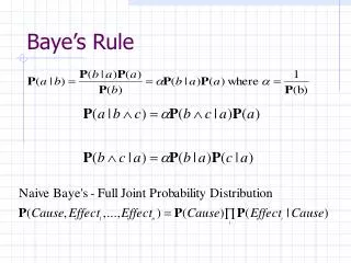
2. Baye’s Rule and Reasoning • Allows use of uncertain causal knowledge • Knowledge: given a cause what is the likelihood of seeing particular effects (conditional probabilities) • Reasoning: Seeing some effects, how do we infer the likelihood of a cause. • This can be very complicated: need joint probability distribution of (k+1) variables, i.e., 2k+1 numbers. • Use conditional independence to simplify expressions. Allows sequential step by step computation

3. Bayesian/Belief Network • To avoid problems of enumerating large joint probabilities • Use causal knowledge and independence to simplify reasoning, and draw inferences

4. Cavity Toothache Catch Weather Bayesian Networks • Also called Belief Network or probabilistic network • Nodes – random variables, one variable per node • Directed Links between pairs of nodes. AB A has a direct influence on B • With no directed cycles • A conditional distribution for each node given its parents Must determine the Domain specific topology.

5. Bayesian Networks • Next step is to determine the conditional probability distribution for each variable. • Represented as a conditional probability table (CPT) giving the distribution over Xifor each combination of the parent value. Once CPT is determined, the full joint probability distribution is represented by the network. The network provides a complete description of a domain.

6. Study Fun Exam College Party Belief Networks: Example • If you go to college, this will effect the likelihood that you will study and the likelihood that you will party. Studying and partying effect your chances of exam success, and partying effects your chances of having fun. • Variables: College, Study, Party, Exam (success), Fun • Causal Relations: • College will affect studying • College will affect parting • Studying and partying will affect exam success • Partying affects having fun.

7. Study Fun Exam College Party College example: CPTs CPT Discrete Variables only in this format

8. Belief Networks: Compactness • A CPT for Boolean variable Xiwith k Boolean parents is 2k rows for combinations of parent values • Each row requires one number p for Xi= true • (the number Xi = false is 1-p) • Row must sum to 1. • Conditional Probability • If each variable had no more than k parents, then complete network requires O(n2k) numbers • i.e., the numbers grow linearly in n vs. O(2n) for the full joint distribution College net has 1+2+2+4+2=11 numbers

9. Study Fun Exam College Party Belief Networks: Joint Probability Distribution Calculation • Global semantics defines the full joint distribution as the product of local distributions: Can use the networks to make inferences. 0.2*0.8*0.4*0.9*0.3 = 0.01728 Every value in a full joint probability distribution can be calculated.

10. Study Fun Exam College Party College example: CPTs 0.2*0.8*0.4*0.9*0.3 = 0.01728

11. Network Construction • Must ensure network and distribution are good representations of the domain. • Want to rely on conditional independence relationships. • First, rewrite the joint distribution in terms of the conditional probability. • Repeat for each conjunctive probability Chain Rule

12. Network Construction • Note is equivalent to: where the partial order is defined by the graph structure. The above equation says that the network correctly represents the domain only if each node is conditionally independent of its predecessors in the node ordering, given the node’s parents. Means: Parents of Xi needs to contain all nodes in X1,…,Xi-1 that have a direct influence on Xi.

13. Study Fun Exam College Party College example: P(F|C, S, P, E) =P(F|P)

14. Compact Networks • Bayesian networks are sparse, therefore, much more compact than full joint distribution. • Sparse: each subcomponent interacts directly with a bounded number of other nodes independent of the total number of components. • Usually linearly bounded complexity. • College net has 1+2+2+4+2=11 numbers • Fully connected domain = full joint distribution. • Must determine the correct network topology. • Add “root causes” first then the variables that they influence.

15. Network Construction • Need a method such that a series of locally testable assertions of conditional independence guarantees the required global semantics • Choose an ordering of variables X1, …., Xn • For i = 1 to n add Xi to network select parents from X1, …, Xi-1 such that P(Xi |Parents(Xi)) = P(Xi | X1,… Xi-1) The choice of parents guarantees the global semantics

16. College Fun Exam Study Party Constructing Baye’s networks: Example • Choose an ordering F, E, P, S, C P(E|F)=P(E)? P(P|F)=P(P)? P(S|F,E)=P(S|E)? P(S|F,E)=P(S)? P(C|F,E,P,S)=P(C|P,S)? P(C|F,E,P,S)=P(C)? Note that this network has additional dependencies

17. College Fun Exam Study Fun Exam College Study Party Party Compact Networks

18. Network Construction: Alternative • Start with topological semantics that specifies the conditional independence relationships. • Defined by either: • A node is conditionally independent of its non-descendants, given its parents. • A node is conditionally independent of all other nodes given its parents, children, and children’s parents: Markov Blanket. • Then reconstruct the CPTs.

19. X Network Construction: Alternative Each node is conditionally independent of its non-descendants given its parents Local semantics  Global semantics Examis independent of College, given the values of Study and Party.

20. Network Construction: Alternative … U1 Um Each node is conditionally independent of its parents, children and children’s parents. – Markov Blanket Z1j X Znj College is independent of fun, given Party. Yn Y1 …

21. Canonical Distribution • Completing a node’s CPT requires up to O(2k) numbers. (k – number of parents) • If the parent child relationship is arbitrary, than can be difficult to do. • Standard patterns can be named along with a few parameters to satisfy the CPT. • Canonical distribution

22. Deterministic Nodes • Simplest form is to use deterministic nodes. • A value is specified exactly by its parent’s values. • No uncertainty. • But what about relationships that are uncertain? • If someone has a fever do they have a cold, the flu, or a stomach bug? Can you have a cold or stomach bug without a fever?

23. Noisy-Or Relationships • A Noisy-or relationship permits uncertainty related to the each parent causing a child to be true. • The causal relationship may be inhibited. • Assumes: • All possible causes are known. • Can have a miscellaneous category if necessary (leak node) • Inhibition of a particular parent is independent of inhibiting other parents. Can you have a cold or stomach bug without a fever? Fever is true iff cold, Flu, or Malaria is true.

24. Example • Given:

25. Example Requires O(k) parameters rather than O(2k) 0.2 * 0.1 = 0.02 0.6 * 0.1 = 0.06 0.6 * 0.2 = 0.12 0.6 * 0.2 * 0.1 = 0.012

26. Networks with Continuous Variables • How are continuous variables represented? • Discretization using intervals • Can result in loss of accuracy and large CPTs • Define probability density functions specified by a finite number of parameters. • i.e. Gaussian distribution

27. Hybrid Bayesian Networks • Contains both discrete and continuous variables. • Specification of such a network requires: • Conditional distribution for a continuous variable with discrete or continuous parents. • Conditional distribution for a discrete variable with continuous parents.

28. Example Continuous child with a discrete parent and a continuous parent Discrete parent Continuous parent subsidy harvest Continuous parent is represented as a distribution. Cost c depends on the distribution function for h. Cost Discrete parent is Explicitly enumerated. A linear Gaussian distribution can be used. Have to define the distribution for both values of subsidy. Buys

29. Example Discrete child with a continuous parent subsidy harvest Set a threshold for cost. Can use a integral of the standard normal distribution. Cost Continuous parent Underlying decision process has a hard threshold but the Threshold’s location moves based upon random Gaussian noise. Probit Distribution Buys Discrete child

30. Example • Probit distribution • Usually a better fit for real problems • Logit distribution • Uses sigmoid function to determine threshold. • Can be mathematically easier to work with.

31. Baye’s Networks and Exact Inference • Notation • X: Query variable • E: set of evidence variables E1,…Em • e: a particular observed event • Y: set of nonevidence variables Y1,…Ym • Also called hidden variables. • The complete set of variables: • A query: P(X|e)

32. Study Fun Exam College Party College example: CPTs

33. Example Query • If you succeeded on an exam and had fun, what is the probability of partying? • P(Party|Exam=true, Fun=true)

34. Inference by Enumeration • From Chap 13 we know: • From this Chapter we have: • P(x,b,y) in the joint distribution can be represented as products of the conditional probabilities.

35. Inference by Enumeration • A query can be answered using a Baye’s Net by computing the sums of products of the conditional probabilities from the network.

36. Example Query • If you succeeded on an exam and had fun, what is the probability of partying? • P(Party|Exam=true, Fun=true) • What are the hidden variables?

37. Example Query • Let: • C = College • PR = Party • S = Study • E = Exam • F =Fun • Then we have from eq. 13.6 (p.476):

38. Example Query • Using we can put in terms of the CPT entries. The worst case complexity of this equation is: O(n2n) for n variables.

39. Example Query • Improving the calculation • P(f|pr) is a constant so it can be moved out of the summation over C and S. • The move the elements that only involve C and not S to outside the summation over S.

40. Study Fun Exam College Party College example:

41. Example Query Similarly for P( pr|e,f). .126 P(f|pr) .9 P(c) .2 + P(pr|c) .6 .06 + .08 = .14 + + P(s|c) .8 .12 + .08 = .2 .48 + .02 = .5 P(e|s,pr) .6 P(e|s,pr) .6 Still O(2n)

42. Variable Elimination • A problem with the enumeration method is that particular products can be computed multiple times, thus reducing efficiency. • Reduce the number of duplicate calculations by doing the calculation once and saving it for later. • Variable elimination evaluates expressions from right to left, stores the intermediate results and sums over each variable for the portions of the expression dependent upon the variable.

43. Variable Elimination • First, factor the equation. • Second, store the factor for E • A 2x2 matrix fE(S,PR). • Third, store the factor for S. • A 2x2 matrix. S C E PR F

44. Variable Elimination • Fourth, Sum out S from the product of the first two factors. • This is called a pointwise product • It creates a new factor whose variables are the union of the two factors in the product. • Any factor that does not depend on the variable to be summed out can be moved outside the summation.

45. Variable Elimination • Fifth, store the factor for PR • A 2x2 matrix. • Sixth, Store the factor for C.

46. Variable Elimination • Seventh, sum out C from the product of the factors where

47. Variable Elimination • Next, store the factor for F. • Finally, calculate the final result

48. Elimination Simplification • Any leaf node that is not a query variable or an evidence variable can be removed. • Every variable that is not an ancestor of a query variable or an evidence variable is irrelevant to the query and can be eliminated.

49. Earthquake MaryCalls JohnCalls Burglary Alarm Elimination Simplification • Book Example: • What is the probability that John calls if there is a burglary? Does this matter?

50. Complexity of Exact Inference • Variable elimination is more efficient than enumeration. • Time and space requirements are dominated by the size of the largest factor constructed which is determined by the order of variable elimination and the network structure.