Optimizing Lattice Boltzmann Flow Simulation for DataFlow Supercomputers: A Software Approach
210 likes | 348 Vues
This work explores the integration of Lattice Boltzmann methods with DataFlow architectures to enhance blood flow simulation performance. We discuss the transition of Lattice Boltzmann (LB) algorithms to Maxeler’s DataFlow systems, outlining existing challenges and presenting a novel software engineering framework. Our approach includes detailed analyses and kernel optimizations, leveraging both static and dynamic data orchestration to achieve significant speed-ups. Collaboration across institutions enhances this study, demonstrating an intricate synergy of physics and software engineering for advanced computational fluid dynamics.

Optimizing Lattice Boltzmann Flow Simulation for DataFlow Supercomputers: A Software Approach
E N D
Presentation Transcript
NenadKorolija, nenadko@etf.rs TijanaDjukic, tijana@kg.ac.rsNenadFilipovic, nfilipov@hsph.harvard.edu VeljkoMilutinovic, vm@etf.rs Lattice Boltzmann for Blood Flow:A Software Engineering Approachfor a DataFlowSuperComputer
MyWork in a NutShell • Introduction: Synergy of Physics and Logics • Problem: Moving LB to Maxeler • ExistingSolutions: None :) • Essence: Map+Opt(PACT) • Details: MyPhD • Analysis: BaU • Conclusions: 1000 (SPC)
Cooperation between BioIRC, UniKG and School of Electrical Engineering, UniBG
Lattice Boltzmann for Blood Flow:A Software Engineering Approach • Expensive • Quiet • Fast • Electrical • 20m cord • Environment-friendly • Big-pack • Wide-track • Easy handling • Reparation manual • Reparation kit • 5Y warranty • Service in your town • New-technology high-quality non-rusting heavy-duty precise-cutting recyclable blades streaming grass only to bag ...
Lattice Boltzmann for Blood Flow:A Software Engineering Approach Expensive Quiet Electrical 20m cord Environment-friendly Big-pack Wide-track Easy handling Reparation manual Reparation kit 5Y warranty Service in your town New-technology high-quality non-rusting heavy-duty precise-cutting recyclable blades streaming grass only to bag ...
Lattice Boltzmann for Blood Flow:A Software Engineering Approach
Structure of the Existing C-Codefor a MultiCore Computer • LS1 LS2 LS3 LS4 LS5 • Statically: P / T = 100 / 400 = 25% => Only 100 lines to “kernelize” • Dynamically: P / T = 99%=> Potential speed-up factor is at most 100 LS – Looping structure LS1 and LS5 – Nested loops LS2, LS3, and LS4 – Simple loops P – lines to parallelize T – total number of lines
What Looping Structures to “Kernelize” • All,because we like all datato reside on MAX3prior to the execution start MAX MAX MAX MAX MAX MAX CPU CPU CPU CPU CPU CPU
What Looping StructuresBring what Benefits? • LS1 moderate • LS2, LS3, LS4negligible,but must “kernelize” • LS5 major FOR i = 1 2 3 4 5 … k … n DO FOR i = 1 2 3 4 5 … n DO T0 T1 T2 T3 T4 T0Tk T2k T3k OP1 OP1 OP2 OP2 OP3 OP3 OP4 OP4 OP5 OP5 OP6 OP6 . . . . . . OPkOPk Tk Tk+1 Tk+2 Tk T2k 1 result/clockMAX T3k T4k 1 result/k*clockCPU DFE doing k operations CPU doing only one
Why “Kernelizing” the Looping Structures?Conditions for “Kernelizing” Revisited
Programming: Iteration #1 What to do with LS1..5? • Direct MultiCore Data Choreography 1, 2, 3, 4, ... • Direct MultiCore Algorithm Execution ∑∑ + ∑ + ∑ + ∑ + ∑∑ • Direct MultiCoreComputational Precision:Double Precision Floating Point (64 bits)
Programming: Iteration #1 Potentials of Direct “Kernelization” • Amdahl Low: limes(DFE Potential → ∞) = 100 • Reality Estimate: limes(work → 30.6.2013.)= N 1% 99% 1% 0% 1% x%
Pipelining the Inner Loops inputs 0 Kernel(s) Stream Middle FunctionsKernels Manager Kernel j Kernel(s) Collide 320 0 112 i output
The Kernel for LS1:Direct Migration • public class LS1Kernel extends Kernel { • public LS1Kernel(KernelParameters parameters) { • super(parameters); • // Input • HWVar f1new = io.scalarInput("f1new" ,hwFloat(8, 24)); • HWVar f5new = io.scalarInput("f5new" ,hwFloat(8, 24)); • HWVar f8new = io.scalarInput("f8new" ,hwFloat(8, 24)); • HWVar f1 = io.input("f1", hwFloat(8, 24)); // j • HWVar f2m = io.input("f2m", hwFloat(8, 24)); // j-1 • HWVar f3 = io.input("f3", hwFloat(8, 24)); // j • HWVar f4p = io.input("f4p", hwFloat(8, 24)); // j+1 • HWVar f5m = io.input("f5m", hwFloat(8, 24)); // j-1 • HWVar f6m = io.input("f6m", hwFloat(8, 24)); // j-1 • HWVar f7p = io.input("f7p", hwFloat(8, 24)); // j+1 • HWVar f8p = io.input("f8p", hwFloat(8, 24)); // j+1
The Kernel for LS5: Direct Migration • // Do the summations needed to evaluate the density and components of velocity • HWVarro = f0 + f1 + f2 + f3 + f4 + f5 + f6 + f7 + f8; • HWVarrovx = f1 - f3 + f5 - f6 - f7 + f8; • HWVarrovy = f2 - f4 + f5 + f6 - f7 - f8; • HWVarvx = rovx/ro; • HWVarvy = rovy/ro; • // Also load the velocity magnitude into plotvar - this is what we will • // display using OpenGL later • HWVar v2x = vx * vx; • HWVar v2y = vy * vy; • HWVarplotvar = KernelMath.sqrt(v2x + v2y); • HWVarv_sq_term = 1.5f*(v2x + v2y); • // Evaluate the local equilibrium f values in all directions • HWVarvxmvy = vx - vy; • HWVarvxpvy = vx + vy; • HWVarrortau = ro * rtau; • HWVar rortaufaceq2 = rortau * faceq2; • HWVar rortaufaceq3 = rortau * faceq3; • HWVar vxpvyp3 = 3.f*vxpvy; • HWVar vxmvyp3 = 3.f*vxmvy; • HWVar vxp3 = 3.f*vx; • HWVar vyp3 = 3.f*vy; • HWVar v2xp45 = 4.5f*v2x; • HWVar v2yp45 = 4.5f*v2y; • HWVarmv_sq_term = 1.f - v_sq_term; • HWVar mv_sq_termpv2xp45 = mv_sq_term + v2xp45; • HWVar mv_sq_termpv2yp45 = mv_sq_term + v2yp45; • HWVar vxpvyp45vxpvy = 4.5f*vxpvy*vxpvy; • HWVar vxmvyp45vxmvy = 4.5f*vxmvy*vxmvy; • HWVar mv_sq_termpvxpvyp45vxpvy = mv_sq_term + vxpvyp45vxpvy; • HWVar mv_sq_termpvxmvyp45vxmvy = mv_sq_term - vxmvyp45vxmvy; • HWVar f0eq = rortau * faceq1 * mv_sq_term; • HWVar f1eq = rortaufaceq2 * (mv_sq_termpv2xp45 + vxp3); • HWVar f2eq = rortaufaceq2 * (mv_sq_termpv2yp45 + vyp3); • HWVar f3eq = rortaufaceq2 * (mv_sq_termpv2xp45 - vxp3); • HWVar f4eq = rortaufaceq2 * (mv_sq_termpv2yp45 - vyp3); • HWVar f5eq = rortaufaceq3 * (mv_sq_termpvxpvyp45vxpvy + vxpvyp3); • HWVar f6eq = rortaufaceq3 * (mv_sq_termpvxmvyp45vxmvy - vxmvyp3); • HWVar f7eq = rortaufaceq3 * (mv_sq_termpvxpvyp45vxpvy - vxpvyp3); • HWVar f8eq = rortaufaceq3 * (mv_sq_termpvxmvyp45vxmvy + vxmvyp3);
Programming: Iteration #2 Ideas for Additional Speedup (a) • Better Data Choreography • 5x x 5x • Estimate: 1.2 X Speed-up (as seen from the drawing above)
Programming: Iteration #3 Ideas for Additional Speedup (b) • Algorithmic Changes:∑∑ + ∑ + ∑ + ∑ + ∑∑ → ∑∑ + ∑ + ∑∑ • Explanation: As seen from the previous drawing,LS2 and LS3 can be integrated with LS1 • Estimate: 1.6
Programming: Iteration #4 Ideas for Additional Speedup (c) • Precision Changes:LUT (Double-precision floating point, 64) = 500LUT (Maxeler-precision floating point, 24) = 24 • Explanation:With less precision,hardware complexity can be reduced by a factor of about 20.Increasing number of iterations 4 timesbrings approximately similar precision, much faster. • Estimate: Factor = (500/24)/4 ≈ 5 • This is the only action,before which an topic expert has to be consulted!
Lattice Boltzman http://www.youtube.com/watch?v=vXpCC3q0tXQ
Results: SPTC≈1000x“Maxeler’s technology enables organizations to speed up processing times by 20-50x,with over 90% reduction in energy usage and over 95% reduction in data centre space”. • Speedup factor: 1.2 x 1.6 x 5 x N ≈ 10N- Precisely 30.6.2013. • Power reduction factor(i7/MAX3) =17.6 / (MAX2 / MAX3) ≈ 10- Precisely: the WallCordmethod • Transistor count reduction factor = i7 / MAX3- Precisely: about 20 • Cost reduction factor: x- Precisely: depends on production volumes
Q&A: nenadko@etf.rs 10km/h ! 30km/h !!! Hawaii Tahiti