Lattices
Lattices. The material in these slides have been taken from the "Dragon Book", and from Michael Schwartzbach's "Lecture Notes in Static Analysis". The Dataflow Framework. We use an iterative algorithm to find the solution of a given dataflow problem.


Lattices
E N D
Presentation Transcript
Lattices The material in these slides have been taken from the "Dragon Book", and from Michael Schwartzbach's "Lecture Notes in Static Analysis".
The Dataflow Framework • We use an iterative algorithm to find the solution of a given dataflow problem. • How do we know that this algorithm terminates? • How precise is the solution produced by this algorithm? My being a teacher had a decisive influence on making language and systems as simple as possible so that in my teaching, I could concentrate on the essential issues of programming rather than on details of language and notation. (N. Wirth) • The purpose of this class is to provide a proper notation to deal with these two questions. • To achieve this goal, we shall look into algebraic bodies called lattices. • But before, we shall provide some intuition on why the dataflow algorithms are correct.
How do we know that liveness terminates? • Given a control flow graph G, find, for each edge E in G, the set of variables alive at E. Can you guess some of the live sets?
Example of Liveness Problem • Let's solve liveness analysis for the program below: Do you remember the dataflow equations that we use to solve liveness?
Dataflow Equations for Liveness • IN(p) = the set of variables alive immediately before p • OUT(p) = the set of variables alive immediately after p • vars(E) = the variables that appear in the expression E • succ(p) = the set of control flow nodes that are successors of p • The algorithm that solves liveness keeps iterating the application of these equations, until we reach a fixed point. • Iff is a function, then p is a fixed point of f if f(p) = p. Why every IN(p) and OUT(p) sets always reach a fixed point?
Dataflow Equations for Liveness • The key observation is that none of these equations take information away of its result. • The result that they produce is always the same, or larger than the previous result. • Given this property, we eventually reach a fixed point, because the INs and OUTs sets cannot grow forever. Can you explain why 1.1 is true? And property 2, why these sets cannot grow forever?
Correctness of Available Expressions • An expression is available at a program point if its current value has already been computed earlier in the execution. Which expressions are available in this example?
Correctness of Available Expressions • An expression is available at a program point if its current value has already been computed earlier in the execution. Do you remember the data-flow equations for this problem?
Dataflow Equations for Availability • IN(p) = the set of expressions available immediately before p • OUT(p) = the set of expressions available immediately after p • pred(p) = the set of control flow nodes that are predecessors of p • Expr(v) = the expressions that use variable v • The argument on why availability analysis terminates is similar to that used in liveness, but it goes on the opposite direction. • Inliveness, we assume that every IN and OUT set is empty, and keep adding information to them. • In availability, we assume that every IN and OUT set contains every expression in the program, and then we remove some of these expressions.
Dataflow Equations for Availability 1) Can you show that each IN and OUT set always decreases? 2) And why can't these sets decrease forever? 3) In the worst case, how long would this system take to stabilize?
Lattices • All our dataflow analyses map program points to elements of algebraic bodies called lattices. • A complete lattice L = (S, ≤, ∨, ∧, ⊥, T) is formed by: • A set S • A partial order ≤ between elements of S. • A least element ⊥ • A greatest element T • A join operator ∨ • A meet operator ∧ Lattice: structure consisting of strips of wood or metal crossed and fastened together with square or diamond-shaped spaces left between, used typically as a screen or fence or as a support for climbing What is a partial order? Can you imagine why we use this name?
Least Upper Bounds and Joins This operator is called "Join" • If L = (S, ≤, ∨, ∧, ⊥, T) is a complete lattice, and e1 ∈ S and e2 ∈ S, then we let elub = (e2 ∨ e1) ∈ S be the least upper bound of the set {e1, e2}. The least upper bound elub has the following properties: • e1 ≤ elub and e2 ≤ elub • For any element e' ∈ S, if e1 ≤ e' and e2 ≤ e', then elub ≤ e' • Similarly, we can define the least upper bound of a subset S' of S as the pairwise least upper bound of every element of S' In order of L to be a lattice, it is a necessary condition that every subset S' of S has a least upper bound elub ∈ S. Notice that elub may not be in S'.
Greatest Lower Bounds and Meets This operator is called "Meet" • If L = (S, ≤, ∨, ∧, ⊥, T) is a complete lattice, and e1 ∈ S and e2 ∈ S, then we let eglb = (e2 ∧ e1) be the greatest lower bound of the set {e1, e2}. The greatest lower bound eglb has the following properties: • eglb ≤ e1 and eglb ≤ e2 • For any element e' ∈ S, if e' ≤ e1 and e' ≤ e2, then e' ≤ eglb • Similarly, we can define the greatest lower bound of a subset S' of S as the pairwise greatest lower bound of every element of S' In order of L to be a lattice, it is a necessary condition that every subset S' of S has a greatest lower bound eglb ∈ S. Notice that eglb may not be in S'.
Properties of Join and Meet • Join is idempotent: x ∨ x = x • Join is commutative: y ∨ x = x ∨ y • Join is associative: x ∨ (y ∨ z) = (x ∨ y) ∨ z • Join has a multiplicative one: for all x in S, (⊥∨ x) = x • Join has a multiplicative zero: for all x in S, (T ∨ x) = T • Meet is idempotent: x ∧ x = x • Meet is commutative: y ∧ x = x ∧ y • Meet is associative: x ∧ (y ∧ z) = (x ∧ y) ∧ z • Meet has a multiplicative one: for all x in S, (T ∧ x) = x • Meet has a multiplicative zero: for all x in S, (⊥∧ x) = ⊥
Joins, Meets and Semilattices • Some dataflow analyses, such as live variables, use the join operator. Others, such as available expressions, use the meet operator. • In the case of liveness, this operator is set union. • In the case of availability, this operator is set intersection. • If a lattice is well-defined for only one of these operators, we call it a semilattice. • The vast majority of the dataflow analyses require only the semilattice structure to work.
Partial Orders • The meet operator (or the join operator) of a semilattice defines a partial order: • This partial order has the following properties: • x ≤ x (The partial order is reflexive) • If x ≤ y and y ≤ x, then x = y (The partial order is antisymmetric) • If x ≤ y and y ≤ z, then x ≤ z (The partial order is transitive) x ≤ y if, and only if x ∧ y = x♧ ♧: For a proof that this equivalence is true, see the "Dragon Book".
The Semilattice of Liveness Analysis • Given the program on the left, we have the semillatice L = (P{x, y, z}, ⊆, ∪, {}, {a, b, c}) • As this is a semilattice, we have only defined the join operator, which, in our case, is set union. • The least element is the empty set, which is contained inside every other subset of {x, y, z} • The greatest element is {x, y, z} itself, which contains every other subset.
Checking the Properties of a Semilattice • Is L = (PS, ⊆, ∪, {}, S) really a semilattice♤? • Is U a join operator? In other words, is it the case that "x ≤ y if, and only if x∨y = y" for ⊆ and U? • We want to know if "x ⊆ y if, and only if, x U y = y" • Is {} a "Least Element"? • The empty set is contained within any other set; hence, for any S' in PS, we have that {} ⊆ S' • Is S a "Greatest Element"? • Any set in PS is contained in S; thus, for any S' in Ps, we have that S' ⊆ S Can you use similar reasoning to show that (PS, ⊇, ∩, S, {}) is also a lattice? ♤: S is any finite set of elements, e.g., S = {x, y, z} in our previous example.
The Semillatice of Available Expressions • Given the program on the left, we have the semillatice L = (P{a+b, a*b, a+1}, ⊇, ∩, {a+b, a*b, a+1}, {}) • As this is a semilattice, we have only defined the meet operator, which, in our case, is set intersection. • The least element is the set of all the expressions (remember, we are dealing with intersection). • The greatest element is the empty set, as it is the intersection of every subset.
Lattice Diagrams • We can represent the partial order between the elements of a lattice as a Hasse Diagram. • If there exists a path in this diagram, from an element e1 to another element e2, then we say that e1 ≤ e2.
Mapping Program Points to Lattice Points The solution of a data-flow problem is a mapping between program points to lattice points.
Lattice Diagrams Which diagrams do not represent lattices?
Transfer Functions • As we have seen in a previous class, the solution of a dataflow problem is given by a set of equations, such as: F(x1, …, xn) = (F1(x1, …, xn), …, Fn(x1, …, xn)) • Each function Fiis a transfer function. • If the dataflow problem ranges over a lattice L, then each Fi is a function of type L → L. Which property must be true about each function Fi and the lattice L, so that a worklist algorithm that solves this system terminates?
Monotone Transfer Functions • We can guarantee that the worklist algorithm that solves the constraint system terminates if these two conditions are valid: • Each transfer function Fi always produces larger results, i.e., given l1 and l2 in the lattice L, we have that if l1≤ l2, then F1(l1) ≤ F1(l2) • Functions that meet this property are called monotone. • The semilattice L must have finite height • It is not possible to have an infinite chain of elements in L, e.g., l0 ≤ l1 ≤ l2 ≤ … such that every element in this chain is different. • Notice that the lattice can still have an infinite number of elements. Can you give an example of a lattice that has an infinite number of elements, and still has finite height?
Monotone Transfer Functions • Let L = (S, ≤, ∨, ∧, ⊥, T), and consider a family of functions F, such that for all f ∈ F, f : L → L. These properties are equivalent*: • Any element f ∈ F is monotonic • For all x ∈ S, y ∈ S, and f ∈ F, x ≤ y implies f(x) ≤ f(y) • For all x and y in S and f in F, f(x ∧ y) ≤ f(x) ∧ f(y) • For all x and y in S and f in F, f(x) ∨ f(y) ≤ f(x ∨ y) * for a proof, see the "Dragon Book", 2nd edition, Section 9.3
Monotone Transfer Functions • Prove that the transfer functions used in the liveness analysis problem are monotonic: • Now do the same for available expressions: prove that these transfer functions are monotonic:
Correctness of the Iterative Solver • We shall show the correctness of a algorithm that solves a forward-must analysis, i.e., an analysis that propagates information from IN sets to OUT sets, and that uses the semilattice with the meet operator. The solver is given on the right: OUT[ENTRY] = vENTRY for each block B, but ENTRY OUT[B] = T while (any OUT set changes) for each block B, but ENTRY IN[B] = ∧p ∈pred(B)OUT[P] OUT[B] = fb(IN[B]) 1) Does this algorithm solve a forward or a backward analysis? 2) How can we show that the values taken by the IN and OUT sets can only decrease?
Induction • Usually we prove properties of algorithms using induction. • In the base case, we must show that after the first iteration the values of each IN and OUT set is no greater than the initial values. • Induction step: assume that after the kth iteration, the values are all no greater than those after the (k-1)st iteration. 1) Why is this statement trivial to show? 2) You need now to extend this property to iteration k + 1
Induction • Continuing with the induction step: • Let IN[B]i and OUT[B]i denote the values of IN[B] and OUT[B] after iteration i • From the hypothesis, we know that OUT[B]k ≤ OUT[B]k-1 • But (2) gives us that IN[B]k+1 ≤ IN[B]k, by the definition of the meet operator, and line 6 of our algorithm • From (3), plus the fact that fb is monotonic, plus line 7 of our algorithm, we know that OUT[B]k+1 ≤ OUT[B]k
The Asymptotic Complexity of the Solver 1: OUT[ENTRY] = vENTRY 2: for each block B, but ENTRY 3: OUT[B] = T 4: while (any OUT set changes) 5: for each block B, but ENTRY 6: IN[B] = ∧p ∈pred(B)OUT[P] 7: OUT[B] = fb(IN[B]) If we assume a lattice of height H, and a program with B blocks, what is the asymptotic complexity of the iterative solver on the right?
The Asymptotic Complexity of the Solver • The IN/OUT set associated with a block can change at most H times; hence, the loop at line 4 iterates H*B times • The loop at line 5 iterates B times • Each application of the meet operator, at line 6, can be done in O(H) • A block can have B predecessors; thus, line 6 is O(H*B) • By combining (1), (2) and (4), we have O(H*B*B*H*B) = O(H2*B3) 1: OUT[ENTRY] = vENTRY 2: for each block B, but ENTRY 3: OUT[B] = T 4: while (any OUT set changes) 5: for each block B, but ENTRY 6: IN[B] = ∧p ∈pred(B)OUT[P] 7: OUT[B] = fb(IN[B]) If we assume a lattice of height H, and a program with B blocks, what is the asymptotic complexity of the iterative solver on the right? This is a pretty high complexity, yet most real-world implementations of dataflow analyses tend to be linear on the program size, in practice.
Fixed Point • The fixed point of a function f:L→L is an element l ∈ L, such that f(l) = l • A function can have more than one fixed point. • For instance, if our function is the identity, e.g., f(x) = x, then any element in the domain of f is a fixed point of it. • Our constraint system on F(x1, …, xn) = (F1(x1, …, xn), …, Fn(x1, …, xn)) stabilizes in a fixed point of F. • If L is a lattice, and f is well-defined for every element e ∈ L, then we have a maximum fixed point. • Similarly, If L is a lattice, and f is well-defined for every element e ∈ L, than we have a minimum fixed point. For each of these three bullets on the right, can you provide a rational on why it is true? In other words, the glb and lub of the fixed points are fixed points themselves.
Maximum Fixed Point (MFP) • The solution that we find with the iterative solver is the maximum fixed point of the constraint system, assuming monotone transfer functions, and a semilattice with meet operator of finite height♧. • The MFP is a solution with the following property: • any other valid solution of the constraint system is less than the MFP solution. • Thus, our iterative solver is quite precise, i.e., it produces a solution to the constraint system that wraps up each equation in the constraint system very tightly. • Yet, the MFP solution is still very conservative. Can you give an example of a situation in which we get a conservative solution? ♧: For a proof, see "Principles of Program Analysis", pp 76-78.
Example: Reaching Definitions • What would be a solution that our iterative solver would produce for the reaching definitions problem in the program below?
Example: Reaching Definitions • What would be a solution that our iterative solver would produce for the reaching definitions problem in the program below? Why is this solution too conservative?
Example: Reaching Definitions • What would be a solution that our iterative solver would produce for the reaching definitions problem in the program below? The solution is conservative because the branch is always false. Therefore, the statement c = 3 can never occur, and the definition d4 will never reach the end of the program.
What would be a wrong solution? More Intuition on MFP Solutions
Wrong Solutions: False Negatives • It is ok if we say that a program does more than it really does. • This excess of information is usually called false positive • The problem are the false negatives. • If we say that a program does not do something, and it does, we may end up pruning away correct behavior
The Ideal Solution • The MFP solution fits the constraint system tightly, but it is a conservative solution. • What would be an ideal solution? • In other words, given a block B in the program, what would be an ideal solution of the dataflow problem for the IN set of B?
The Ideal Solution • The MFP solution fits the constraint system tightly, but it is a conservative solution. • What would be an ideal solution? • In other words, given a block B in the program, what would be an ideal solution of the dataflow problem for the IN set of B? • The ideal solution computes dataflow information through each possible path from ENTRY to B, and then meets/joins this info at the IN set of B. • A path is possible if it is executable.
The Ideal Solution • Each possible path P, e.g.: ENTRY → B1 → … → BK → B gives us a transfer function fp, which is the composition of the transfer functions associated with each Bi. • We can then define the ideal solution as: IDEAL[B] = ∧p is a possible path from ENTRY to Bfp(vENTRY) • Any solution that is smaller than ideal is wrong. • Any solution that is larger is conservative.
The Meet over all Paths Solution • Finding the ideal solution to a given dataflow problem is undecidable in general. • Due to loops, we may have an infinite number of paths. • Some of these paths may not even terminate. • Thus, we settle for the meet over all paths (MOP) solution: MOP[B] = ∧p is a path from ENTRY to Bfp(vENTRY) Is MOP the solution that our iterative solver produces for a dataflow problem? What is the difference between the ideal solution and the MOP solution?
Distributive Frameworks♥ • We say that a dataflow framework is distributive if, for all x and y in S, and every transfer function f in F we have that: f(x∧y) = f(x) ∧ f(y) • The MOP solution and the solution produced by our iterative algorithm are the same if the dataflow framework is distributive♣. • If the dataflow framework is not distributive, but is monotone, we still have that IN[B] ≤ MOP[B] for every block B Can you show that our four examples of data-flow analyses, e.g., liveness, availability, reaching defs and anticipability, are distributive? ♥ We are considering the meet operator. An analogous discussion applies to join operators. ♣ For a proof, see the "Dragon Book", 2nd edition, Section 9.3.4
Distributive Frameworks Our analyses use transfer functions such as f(l) = (l \ lk) ∪ lg. For instance, for liveness, if l = "v = E", then we have that IN[l] = OUT[l] \ {v} ∪ vars(E). So, we only need a bit of algebra: f(l ∧ l') = ((l∧ l') \ lk)∪lg(i) ((l \ lk ∧ l' \ lk))∪lg(ii) ((l \ lk) ∪ lg)∧ ((l' \ lk) ∪ lg) (iii) f(l) ∧ f(l') (iv) To see why (ii) and (iii) are true, just remember that in any of the four data-flow analyses, either ∧ is ∩, or it is ∪.
Ascending Chains Our constraint solver finds solutions starting from a seed s, and then computing elements of the underlying lattice that are each time larger than s, until we find an element of this lattice that satisfies the constraints. We find the least among these elements, which traditionally we call the system's Maximum Fixed Point.
Map Lattices • If S is a set and L = (T, ∧) is a meet semilattice, then the structure Ls = (S → T, ∧s) is also a semilattice, which we call a map semilattice. • The domain is S → T • The meet is defined by f ∧f' = λx.f(x) ∧f'(x) • The ordering is f ≤ f' ⇔ ∀x, f(x) ≤ f'(x) • A typical example of a map lattice is used in the constant propagation analysis.
Constant Propagation • How could we optimize the program on the left? • Which information would be necessary to perform this optimization? • How can we obtain this information?
Constant Propagation What is the lattice that we are using in this example?
Constant Propagation • We are using a map lattice, that maps variables to an element in the lattice L below: How are the transfer functions, assuming a meet operator?
Constant Propagation: Transfer Functions • The transfer function depends on the statement p that is being evaluated. I am giving some examples, but a different transfer function must be designed for every possible instruction in our program representation: How is the meet operator, e.g., ∧, defined?