Download
1 / 40
400 likes | 500 Vues
Learn about NP-complete problems, polynomial reduction, and transformations in computer science. Explore key concepts and propogations.

E N D
6. The Most Difficult NP Problems: The Class NPC • Polynomial transformation: Given Xi = (Di , Fi), i = 1, 2 function g : D1 D2 such that g(d) F2 iff d F1. If the function g is computable in time that is polynomial in the length of the encoding of d, then X1 is said to be polynomially transformable to X2. (notation: X1 X2 , L1 L2 ( in language term)) • Note that X1 X2 means that X2 is no easier than X1 in terms of polynomial time solvability. If we can solve X2 in polynomial time (find ‘yes’, ‘no’ answer using deterministic algorithm), then we can answer whether any given instance of X1 is ‘yes’ or ‘no’ in polynomial time. But, the converse may not hold.
Polynomial reduction: X1 is polynomially reducible to X2 if algorithm for X1 that uses algorithm for X2 as a subroutine and runs in polynomial time assuming each call to the subroutine takes unit time. ( recall Opt and Feas for 0-1 IP problem) ( transformation is the special case of reduction) • Polynomial transformation also called Karp reduction, (GJ). Polynomial reduction called Turing reduction, T (GJ). • Prop: If X1 is polynomially transformable (reducible) to X2 , and X2 P, then X1 P. • Def: X1 is a special case of X2 if D1 D2 and F1 = D1 F2. ( Use identity transformation g(d) = d.)
Def: X NP is said to be NP-complete if all problems in NP can be polynomially reduced (transformed) to X. The set of NP-complete problems is denoted by NPC. • NP-complete problem is the hardest problem in NP since the existence of a polynomial time algorithm for any NP-complete problem implies that all the problems in NP can be solved in polynomial time. • Prop 6.3: If X is NP-complete, then P = NP iff X P. ( P NPC P = NP ) Pf) XNP and P = NP XP. X P NPC poly time alg. for any problem in NP. Hence NP P. Also PNP. So P=NP. • Prop 6.4: If X1 is NP-complete, X1 X2 and X2 NP, then X2 is NP-complete. ( Be careful about the direction of the transformation.)
Is NPC ? • First NP-complete problem found: Satisfiability problem (Cook, 1971) Given a set U of Boolean variables and a collection C of clauses over U, is there a satisfying truth assignment for C? ( Is there a truth assignment to i C { j = 1ni ( uj or uj ) } ? ) ( : and, : or ) ex) Given ( u1 u3 ) (u1 u2 u3 ) ( u2 u3 ), a truth assignment is u1 = true, u2 = false, u3 = false • Thm 6.5: (Cook) The satisfiability problem (SAT) is NP-complete. Pf) polynomial transformation of any NDTM into the satisfiability problem. (GJ, pp.38-44)
Prop 6.6: 0-1 IP feasibility problem is NP-complete. Pf) clearly in NP. Let each clause be Ci = ( Ci+, Ci- ). Then (SAT) is satisfiable iff is feasible. We have a function that transforms any instance of (SAT) to an in stance of 0-1 IP feasibility. • Note that we transform an arbitrary instance of (SAT) to a (specific) instance of 0-1 IP feasibilty, which depends on the given instance of (SAT). The rationale is that if there exists an efficient algorithm to solve any instance of 0-1 IP feasibility, we can apply the algorithm to the transformed instance to solve any arbitrary instance of (SAT). So it is unlikely that such efficient algorithm for 0-1 IP feasibility exists since the existence of such algorithm implies that we can solve (SAT) easily and solve all problems in NP easily.
Boundary between P and NPC: { x Bn : Ax b, cx z } ? A: m n 0-1 matrix. • two 1’s in each column of A (node-edge incidence matrix) : matching problem P • Three 1’s in each column NPC • One 1 in each row P • Two 1’s in each row (edge-node incidence matrix) : node packing problem NPC • Be careful about the distinction between the feasibility problem itself and the 0-1 IP formulation.
Unweighted node packing problem (independent set, stable set): Given a graph G = (V, E), U V such that |U| k and U is a node packing? • Prop 6.7: The lower bound feasibility problem for unweighted node packing is NP-complete. Pf) in NP. transform from (SAT) ex) Ci+ Ci- 1 {1, 2} {3} 2 {2, 3} {4} 3 {4} {1, 2} 4 {3} clauses = m, vars = n set k = m {1, 3} = ‘true’, {2, 4} = ‘false’ (1, 1) (5, 3) (2, 1) (7, 1) (6, 3) (3, 4) (3, 2) (4, 3) (8, 2) (2, 2)
Then the given instance of (SAT) has truth assignment iff node packing of size k. • Note that k is set depending on the given instance of (SAT). It is not an arbitrary number. • If we want to claim that IP feasibility formulation of node packing lower bound feasibility is NP-complete, we need to transform the node packing to the IP formulation.
Clique: Given G = (V, E), U V is called a clique if v, w U (v, w) E. (complete subgraph of G) • Clique problem: Given G = (V, E) and positive integer k, a clique of size k ? • Prop: Clique problem is NP-complete Pf) in NP. Independent set (node packing) clique Given an instance of node packing (G, k), construct Gc = (V, E), E = { (i, j) : (i, j) E, i, j V }. Set k = k Then U V is an independent set for G iff U is a clique for Gc. Hence G has an independent set of size k iff Gc has a clique of size k.
Vertex cover: Given G = (V, E), U V is called a vertex cover if all edges in G are incident to at least one vertex in U. • Vertex cover problem:Given G = (V, E), a vertex cover of size k ? (NP-complete) Pf) in NP. clique vertex cover Given an arbitrary instance of clique (G, l), construct an instance of vertex cover. Construct Gc and set k = |V| - l. Then U V is a clique of size k in G V\U is a vertex cover of size n-k in Gc. ) nodes in U not connected by edges in Gc. edges in Gc incident to at least on node in V\U. V\U vertex cover in Gc. ) every edge in Gc is incident to at least one node in V\U no edge in Gc connects nodes in U. U clique in G.
Relation between node packing (independent set), clique, vertex cover: G = (V, E), U V • U is a vertex cover for G. • V\U is a node packing for G. • V\U is a clique in Gc.
Six Basic NP-complete Problems (GJ) • 3-Satisfiability (3SAT) Instance: Collection C = { c1, c2, … , cm } of clauses on a finite set U of variables such that | ci | = 3 for 1 i m. Question : Is there a truth assignment for U that satisfies all the clauses in C ? • 3-Dimensional Matching (3DM) Instance : A set M W X Y, where W, X, and Y are disjoint sets having the same number q of elements. Question : Does M contain a matching, that is, a subset M’ M such that |M’| = q and no two elements of M’ agree in any coordinate ? (generalization of marriage problem.)
Vertex Cover • Clique • Hamiltonian Circuit: Instance : A graph G = (V, E) Question : Does G contain a Hamiltonian circuit, that is, an ordering < v1, v2, … , vn > of the vertices of G, where n = |V|, such that {vn, v1} E and {vi, vi+1 } E for all i, 1 i < n ? • Partition: Instance : A finite set A and a “size” s(a) Z+ for each a A. Question : Is there a subset A’ A such that a A’ s(a) = a A - A’ s(a) ?
Proving NP-completeness • Set partitioning feasibility problem : Given an m n 0-1 matrix A, is {x Bn : Ax = 1 } ? • Prop 6. 8: Set partitioning feasibility problem is NP-complete. Pf) In NP. Lower bound feasibility problem for unweighted node packing Set partitioning feasibility problem Given an instance of node packing (G, k), let A be ( |E|+k) ( |E|+k|V|) matrix defined as follows. = [ B0, B1, B2, … , Bk ] ( AG is edge-node incidence matrix of G.)
Ax = 1 feasible pick k distinct columns of AG’s node packing of size k. Similarly, for converse. Hence k node packing of G set partitioning feasible with k columns (variables) = 1 • Prop 6. 9: The set partitioning feasibility feasibility problem in which matrix A has, at most, three 1’s per column is NP-complete.
2 e1 e3 • Ex) e4 1 3 e5 e2 4 A =
Subset sum problem: Given an integer n, integral n-vector (a1, … , an ), and integer b, is {x Bn : j N aj xj = b } ? • Prop 6.10: The subset sum problem is NP-complete. Pf) in NP. Set partitioning feasibility problem subset sum. Given an m n 0-1 matrix A, construct an instance of subset sum as follows. ( j-th column of A is representation of aj using (n+1) symbols.)
0-1 knapsack lower bound feasibility problem: Given an integer n, integral n-vectors (a1, … , an) and (c1, … , cn), and integers b and z, is {x Bn : j N aj xj b, j N cj xj z } ? (NP-complete) Pf) in NP. Subset sum problem can be reformulated as {x Bn : j N aj xj b, j N aj xj b }. Hence it is a special case of 0-1 knapsack lower bound feasibility. Since special case is NP-complete, more general case is NP-complete. ( recall the definition of special case. It is identity transformation ( or any obvious one-to-one correspondence between the instances.) (special case also called “restriction” and one of the easiest and widely used proving techniques.) • Note that 0-1 knapsack is not a special case of integer knapsack.
More examples of Restriction • Variants of Hamiltonian Circuit : • Hamiltonian Path: Same as HC except that we drop the requirement that the first and the last vertices in the sequence be joined by an edge. • Hamiltonian Path between Two Points: same as HP except that two points u, v are given as input and the question is whether G contains a HP beginning with u and ending with v. • All three problems NP-complete • For directed graph ? transform each undirected problem to a directed problem by replacing each edge of G by two parallel arcs of opposite direction. Undirected version is a special case of directed version.
Bounded Degree Spanning Tree : Instance : A graph G = (V, E) and a positive integer k |V| - 1. Question : Is there a spanning tree for G in which no vertex has degree exceeding k, that is, a subset E’ E such that |E’| = |V| - 1, the graph G’ = (V, E’) is connected, and no vertex in V is included in more than k edges from E’ ? Restrict to Hamiltonian Path by allowing only instances in which k = 2. HP is a special case of BDST with k = 2.
Multiprocessor Scheduling: Instance : A finite set A of ‘tasks’, a ‘length’ l(a) Z+ for each a A, a number m Z+ of ‘processors’, and a ‘deadline’ D Z+. Question : Is there a partition A = A1 A2 … Am of A into m disjoint sets such that max { a Ai l(a) : 1 i m } D ? Restrict to partition by allowing only instances in which m = 2 and D = ½ a A l(a)
Longest Path: Instance : Graph G = (V, E), positive integer k |V| Question : Does G contain a simple path ( that is, a path encountering no vertex more that once) with k or more edges ? Restrict to Hamiltonian Path, i. e. set k = |V|-1 • Set Packing: Instance : Collection C of finite sets, positive integer k |C| Question : Does C contain k disjoint sets ? Restrict to Exact Cover by 3-Sets, i. e. restrict |c| = 3, for all c C and k = q.
Exact Cover by 3-Sets (X3C): (NP-complete) Instance : A finite set X with |X| = 3q and a collection C of 3-element subsets of X. Question : Does C contain an exact cover for X, that is, a subcollection of C’ C such that every element of X occurs in exactly one member of C’ ? Note that 3DM is a restricted version of X3C, hence X3C is NP-complete. Compare to NW p115, 117 in representing the problems.
Proving Traveling Salesman Problem is NP-complete. Instance : Set C of m cities, distance d(ci , cj ) Z+ for each pair of cities ci , cj C, a positive integer B. Question : Is there a tour of C having length B or less, i.e., a permutation < c(1), c(2), … , c(m) > of C such that [ i = 1m-1 d( c(i), c(i+1) ) ] + d( c(m), c(1) ) B ? Pf) In NP. HC TSP Given G = (V, E), construct an instance of TSP as follows. Let ci = vi , vi V. Let d(ci , cj ) = 1 if (vi , vj ) E and = 2 if (vi , vj ) E. Set B = |V|. Then G has a HC iff TSP has a tour B.
If P NP, then NPC P NP. ( i.e. there are problems of intermediate difficulty.) NP \ ( P NPC) is called NPI (Intermediate) • Note • Members in NPI not equivalent in terms of polynomial transformation. ( infinite number of equivalent classes.) • Only artificial examples known. Have been looking for natural problems in NPI. • Composite number, LP regarded as candidates in NPI. • Composite Number : Given positive integer k, are there integers m, n > 1 such that k = mn
Note that composite number is in NP and its complementary problem (Primes) is to check the primality of a given prime number. There exists a short proof to check primality. Hence Composite Number is in NP CoNP. So it is unlikely that composite number is NP-complete by Prop 6.12. Composite number was proven to be in P in 2002. NP NPC NPI P
CoNP NP NPC • Prop 6. 12: If NPC CoNP , then NP = CoNP ( It is unlikely that any problem in NP CoNP is NP-complete) Pf) If X NP there exists polynomial transformation g such that X Y for Y NPC CoNP Since Y CoNP, Y NP. For an instance in X, g maintains ‘yes’ ‘no’ answer after the transformation. If a ‘no’ instance in X is given, we can apply g to it, and obtain an instance in Y which has ‘no’ answer. Since Y NP, we can verify the ‘no’ by polynomial time NDTM. So ‘no’ instance in X can be verified XCoNP NP CoNP Similarly, for the other direction. P
Status of Open Problems in GJ • Source : Pulleyblank, MPS 2000 tutorial • 1. Graph Isomorphism open 2. Subgraph homeomorphism for a fixed graph P 3. Graph genus NP-complete 4. Chordal graph completion NP-complete 5. Chromatic index NP-complete 6. Spanning tree parity P 7. Partial Order Dimension NP-complete 8. Precedence constrained 3-processor schedu open 9. Linear Programming P 10. Total Unimodularity P 11. Composite number open (P) 12. Minimum length triangulation open
NP-complete in the strong sense (strongly NP-complete) • Refer GJ. p90 - • Recall that O(nb) algorithm for 0-1 knapsack problem (also subset sum). Though 0-1 knapsack feasibility is NP-complete, O(nb) is less formidable than O(2n). If b is small (polynomial of n), the algorithm runs in polynomial time for the restricted case. called pseudo-polynomial time algorithm. • Q) pseudo-polynomial time algorithms for other NP-complete problems involving numbers like b? e.g.) TSP feasibility, Multiprocessor scheduling. • Problems like clique, vertex cover do not have pseudo-polynomial time algorithms. • Some problems involving numbers do not have even pseudo-polynomial time algorithms.
For each instance I of decision problem D, define the functions Length[ I ]: length of encoding of I. Max[ I ]: magnitude of largest number in I. (not the size of encoding) • Def: An algorithm for is called a pseudo-polynomial time algorithm for if its time complexity function is bounded above by a polynomial function of Length[ I ] and Max[ I ]. (In NW, polynomial running time in unary encoding ) • Def: A problem is called a number problem if there exists no polynomial p such that Max[ I ] p( Length[ I ]) for all I D e.g) knapsack, partition
Let p be subproblem of restricted to instances such that Max[ I ] p( Length[ I ]) . Then if pseudo-polynomial time algorithm for p solvable in polynomial time. • Def: A decision problem is NP-complete in the strong sense (strongly NP-complete)if is in NP and there exists a polynomial function p for which p is NP-complete. It is the problem class for which there might not exist even pseudo-polynomial time algorithms. If a problem is not a number problem and NP-complete, then it is automatically strongly NP-complete. • NW: Feasibility problem X is called strongly NP-complete if the existence of a pseudo-polynomial time algorithm for it implies P = NP.
Ex) 0-1 IP feasibility with coefficients 0, +1, -1 (transformation from satisfiability, size of numbers in r.h.s. also small) TSP: HC TSP. Edge weights 1 or 2 B = |V|. Hence, all instances with this transformation satisfy Max[ I ] p(Length[ I ]) and NP-complete. So TSP is strongly NP-complete ( Length[ I ] = |V| + log|V| + log d(I, j) ) 3-Partition: Instance: A finite set A of 3m elements, a bound B Z+, and a ‘size’ s(a)Z+ for each aA, such that s(a) satisfies B/4 < s(a) < B/2 and such that aA s(a) = mB. Question : Can A be partitioned into m disjoint sets S1, S2, … , Sm such that, for 1 i m, aSi s(a) = B ?
Multiprocessor Scheduling Sequencing within intervals: Instance: A finite set T of ‘tasks’ and, for each t T, an integer ‘release time’ r(t) 0, a ‘deadline’ d(t) Z+, and a ‘length’ l(t) Z+. Question: Does there exist a feasibleschedule for T, that is, a function : T Z+ such that, for each t T, (t) r(t), (t) + l(t) d(t), and, if t’ T-{t}, then either (t’) + l(t’) (t) or (t’) (t) + l(t) ?
Proving strong NP-completeness by considering restricted problem may be tedious. Use pseudo-polynomial transformation from a strongly NP-complete problem. • Def: A pseudo-polynomial transformation from to ’ is a function f : D D’ such that • For all I D , I Y if and only if f(I) Y’ , • f can be computed in time polynomial in the two variables Max[ I ] and Length[ I ], • a polynomial q1 such that, for all I D , q1 (Length’[ f(I) ] ) Length[ I ] ( size of transformed length does not shrink too much.) • a two variable polynomial q2 such that, for all I D , Max’[ f(I) ] q2 ( Max[ I ] , Length[ I ] ) ( magnitude of the largest number does not blow up exponentially)
Lemma: If is NP-complete in the strong sense, ’ NP, and there exists a pseudo-polynomial transformation from to ’, then ’ is NP-complete in the strong sense. • Note that the transformation from set partitioning feasibility (which is strongly NP-complete) to subset sum is not a pseudo-polynomial transformation. Max’[ f(I) ] ( b = {(n+1)m – 1}/n ) is not bounded by any poly function of Length[ I ] ( mn ). Hence the existence of pseudo-polynomial time algorithm for subset sum cannot be ruled out. Also, if X is NP-complete and X Y, and if there exists a pseudo-polynomial time algorithm for Y, it does not necessarily imply the existence of a pseudo-polynomial time algorithm for X.
NP-hard Problems • GJ Chapter 5 • Search problem : Given an instance I D , return string s, such that s S [ I ] or decide no such string s exists. (S [I ]: set of solutions for I) ( Decision problem may be regarded as a special case of search problem by defining S [I ] ={‘yes’} if I Y and S [I ] = if I Y ) • Def: A polynomial time Turing reduction (or simply Turing reduction) from a search problem to a search problem ’ is an algorithm A that solves by using a hypothetical subroutine S for solving ’ such that, if S were a polynomial time algorithm for ’, then A would be a polynomial time algorithm for (the subroutine may be used many times and and ’ need not be feasibility problems)
Def: A search problem is NP-hard if there exists an NP-complete problem ’ such that ’ T (Turing reducible) ( is at least as hard as NP-complete problem ’ and is search problem (optimization problem) • Recall (0-1 IP FEAS) T (0-1 IP OPT) • Def:A search problem is called NP-easy if there exists a ’ NP such that T ’ ( search problem is no harder than NP-complete problems. Recall (0-1 IP OPT) T (0-1 IP FEAS) )
A search problem is called NP-equivalent if both NP-hard and NP-easy. (has the same degree of difficulty as an NP-complete problem in terms of polynomial time solvability.) To show that an optimization problem is difficult to solve (NP-hard), it is enough to show that the corresponding feasibility problem is NP-complete and the optimization problem is Turing reducible from the feasibility problem (usually trivial). Some people use the term NP-complete for optimization problems too.
Optimization and Separation • Relates the complexity of a class of optimization problem over certain polyhedra with the separation problem for the polyhedra. • Optimization, separation trivial if A: mn is given explicitly. But if polyhedron is given as conv(X) where X is set of feasible solutions, the story is different. ex) x* conv(X)? for node packing is nontrivial if x* is fractional. • Separation problem: Given x* Rn, is x* conv(X)? If not, find an inequality x 0 satisfied by all points in X, but violated by the point x*.
Thm: Optimization problem over a class of polyhedra is polynomially solvable if and only if the separation problem for the polyhedra is polynomiallly solvable.