Download
1 / 28
280 likes | 462 Vues
On approximating a geometric prize-collecting traveling salesman problem with time windows. Reuven Bar-Yehuda Guy Even Shimon (Moni) Shahar. 1.5 hours. 4 hours. 2 hours. 2 hours. 2 hours. 1 hour. 1 hour. 1 hour. Motivation – nurse visiting patients. 10:00-11:00. 6:00-7:00.

E N D
On approximating a geometric prize-collecting traveling salesman problem with time windows Reuven Bar-Yehuda Guy Even Shimon (Moni) Shahar
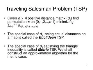
1.5 hours 4 hours 2 hours 2 hours 2 hours 1 hour 1 hour 1 hour Motivation – nurse visiting patients 10:00-11:00 6:00-7:00 12:00-8:00 16:00-17:00 0.5 hour rest 17:00-18:00 7:00-5:00 7:00-6:00 12:00-8:00 leave home at 5:00 get back at 20:00
Prize-collecting TSP with time windows • Definition: • Sites in a metric space (e.g. the plane). • A time-interval for each site (release-time, deadline). • Moving agent with speed in [0,1]. • Goal: max #sites the agent visits on-time. • Extra: service-time per site.
Known results: scheduling with locations • Feasibility is NPC even for points on a line [Tsitsiklis92]. • Polynomial algorithm for the case where all intervals are [0,t_i] (using dynamic programming) [Khanna] • Min makespan (completion time of last job): • 1.5-approx for points on a line with release times, processing times, and no deadlines [KNI98]. • 2-approx for points on a line, no deadlines, multiple agents (vehicles) [KN01]. • PTAS for trees with O(1) leaves, single & multiple agents [AS02].
Our results • Logarithmic approximation for points on a line. • Optimal algorithm for points in any metric space, for special case: no round-trips within time windows. • Heuristic for any metric space. Achieves an approximation ratio that depends on a “density” measure.
t Points on a line • Speed in [0,1], so dist(A,B) = amount of time required to travel from A to B. • Construct the following 2D view of an instance: • speed = 1/slope Slope in 900+[-450,+450] Simplify tour: discrete speed in {-1,0,1}. X
t-X t+X Point on a line (cont.) • Now we rotate the view by 450, and obtain a weakly x-monotone tour {00,450,900}. 2-D generalization of the “max monotone subsequence” problem
1 1 1 1 1 1 2 1 1 1 1 1 1 An 8-approx for unit intervals • Construct a 1/2 -square grid. • Each interval intersects exactly 2 grid lines. • Direct the grid up & right. • Assign edge weights (#intersecting intervals). • Find a longest path on the obtained DAG. An instance (slanted intervals in the plane).
Cj Ci Analysis - definitions • horizontal slice is the region defined by two consecutive horizontal lines. • vertical slice is the region defined by two consecutive vertical lines. • Ci dominates Cj if: • Right(Ci) Left(Cj) && • Top (Ci) Bott(Cj) • Domination ensures that concatenation of sub-tours is feasible.
Segment counted twice Analysis (cont.) THM: The longest path in the graph intersects no less than OPT/8 intervals. • Each interval intersects 2 grid-segments • weight(path) : wrong by at most a factor of 2.
Optimal path Analysis (cont.) “decompose” OPT into alternating horizontal and vertical blocks. (each block within a slice). • Sub-tours through red (blue) blocks can be concatenated. • If there is a grid-path that is 4-approx in each block, pick red or blue blocks. This gives an 8-approx.
OPT in a block Analysis (cont.) Select either left-top path or bottom-right path in the DAG. Every interval in block must intersect the perimeter OPT intersects at most 2 times more intervals than the better path. Error in weight of path is at most by a factor of 2. Overall: 8-approximation
Remarks • For [1,2) intervals this is a 16-apx algorithm. • This can be extended to a 16log(I)-approx. alg. for arbitrary intervals, where I = Imax/Imin. • The size of the DAG is weakly polynomial. It becomes strongly poly if we consider only grid lines that intersect some interval.
An O(log n) approximation • If I = Imax/Imin is is super-poly, then O(log I)> O(log n). • We need a different approach to divide the intervals into “disjoint-sets”. • We use an interval tree for this partition.
Recursive bisection Claim: separating vertical line (at most half the intervals lie strictly on each side).
Level 2 Level 2 2nd comb Recursive bisection (cont.) • A comb defines subset of intervals that intersect exactly one comb-tooth. • bisect recursively log(n) “combs” • comb Ci such that: Ci OPT contains at least OPT/log n intervals. Level 1
O(log(n)) Approximation • Partition the intervals into (log n) combs. • For each comb, 12-approximate an optimal tour. • O(log(n)) approximation.
Approximation for comb • Construct a DAG. • Form a grid. • Find the longest path. • An interval crosses exactly 1 vertical line. • An interval can cross many horz lines (but a grid-path crosses at most 2).
Approx ratio = 12 • Decompose OPT into alternating sub-tours: • horizontal sub-tours inside a slice • vertical sub-tours between two comb teeth • Note the slices are non-uniform, but the proof still holds.
No round-trips within time windows DEF: • for all pairs (vi,vj): dist(vi,vj) + dist(vj,vi) > interval (vi). • Service time: dist(vi,vj) + dist(vj,vi) + serv(vj) > interval(vi). IDEA: can’t zig-zag between sites.
Dynamic program for no round-trips within time windows Intuition: examine two tours A,B such that: • Both visit k sites • Both end at site vi. • tour A ends at time tA. • tour B ends at time tB. • tA < tB • A+best-aug(A) B+best-aug(B) • Proof: aug(B) is also aug(A). Prize-collecting is additive because aug(B) cannot visit sites visited by A.
Dynamic program for no round-trips within time windows (cont.) The algorithm works in layers, where in each layer, it keeps a list of states. A state in layer i is a pair (v,t) which signifies: a path that ends in v at time t after visiting i sites. • Layer 0: (origin, t=0)
Dynamic program for no round-trips within time windows (cont.) • Layer i+1 (induction step): For each state (vi,t) in Layer i go from (vi ,t) to all vj. • Consider the state (vj,t+dist(vi,C) • After deadline? Don’t add to layer i+1. • On time? is it earlier than previous states that end in vj ? If so replace. • Before release time? Use release time instead of arrival time.
Analysis of the dynamic program • Correctness: lexicographic order all optimal tours by considering vector of service times. observation: algorithm computes an optimal tour that is minimal in this order. Running time: • each layer has at most one interesting point per interval. • each point produces at most n candidates for next layers. • number of layers is at most n. The running time is O(n3).
Generalized no-round trip • The density of an instance is: () = maxuv {I(u) / (Luv + Lvu) } • Density bounds number of zig-zags. • The approximation ratio of the dynamic program is: () +1. • This follows from the fact that between every two visits of the same site, at least 1/ () of its length passed. • Non-unit profits: the problem is knapsack hard, and an approximation scheme of (1+) is possible.
Remarks • This algorithm works also for asymmetric distances. • It shows that difficulty is due to “close” intervals.
Further research • Improve approximation ratio in 1-D. • Nothing known for 2-D.