Download
1 / 33
350 likes | 604 Vues
Simulation in Digital Communication. By: Dr. Uri Mahlab. Chapter # 2 Random Processes. By: Dr. Uri Mahlab. Generation of Random Variables. Most computer software libraries include a uniform random number generator. Such a random number generator a number

E N D
Simulation in Digital Communication By: Dr. Uri Mahlab
Chapter # 2 Random Processes By: Dr. Uri Mahlab
Generation of Random Variables • Most computer software libraries include a • uniform random number generator. • Such a random number generator a number • between 0 and 1 with equal probability. • We call the output of the random number • generator a random variable. • If A denotes such a random variable, its • range is the interval
Is called the probability density function F(A) is called the probability distribution function Where:
F(A) f(A) 1 1 A A 0 1 0 1 Fig 1 (a) (b) Figure: Probability density function f(A) and the probability distribution function F(A) of a uniformly distributed random variable A.
If we wish to generate uniformly distributed noise in an interval (b,b+1), it can be accomplished simply by using the output A of the random number generator and shifting it by an amount b. Thus a new random variable B can be defined as Which now has a meanvalue
F(B) f(B) 1 1 B B 0 0 (b) (a) Fig 2 Figure : Probability density function and the probability distribution function of zero- mean uniformly distributed random variable
F(C) 1 A=f(C) C C 0 Fig.3 Figure : Inverse mapping from the uniformly distributed random variable A to the new random variable C
Example 2.1Generate a random variable C that has the linear probability density function shown in Figure (a);I.e., F(C) f(C) 1 1 C C 0 2 (b) 0 2 Fig - 4 (a) Figure : linear probability density function and the corresponding probability distribution function Answer ip_02_01
Thus we generate a random variable C with probability function F(C) ,as shown in Figure 2.4(b). In Illustartive problem 2.1 the inverse mapping C= (A) was simple. In some cases it is not. • Lets try to generate random numbers that have a normal distribution function. • Noise encountered in physical systems is often characterized by the normal,or Gaussian probability distribution, which is illustrated in Figure 2.5. The probability density function is given by Gaussian Normal Noise
F(C) f(C) 1 C C Fig 5 0 0 (b) (a) Gaussian probability density function and the corresponding probability distribution function.
Unfortunately,the integral cannot be expressed in terms of simple functions. Consequently the inverse mapping is difficult to achieve. A way has been found to circumvent this problem. From probability theory it is known that a Rayleigh distributed random variable R, with probability distribution function
Is related to a pair of Gaussian random variables C and D through the transformation
Where A is a uniformly distributed random variable in the interval(0,1). Now, if we generate a second uniformly distributed random variable B and define Then from transformation,we obtain two statistically independent Gaussian distributed random variables C and D.
Gaussian Normal Noise u=rand; % a uniform random variable in (0,1) z=sgma*(sqrt(2*log(1/(1-u)))); % a Rayleigh distributed random variable u=rand; % another uniform random variable in (0,1) gsrv1=m+z*cos(2*pi*u); gsrv2=m+z*sin(2*pi*u); Gngauss.m
Example 2.2: [Generation of samples of a multivariate gaussian process] Generate samples of a multivariate Gaussian random process X(t) having a specified mean value mx and a covarianceCx Answer ip_02_02
Example 2.3: generate a sequence of 1000(equally spaced) samples of gauss Markov process from the recursive relation Answer ip_02_03
Power spectrum of random processes and white processes A stationary random process X(t) is characterized in the frequency domain by its power spectrum which is the fourier transform of the autocorrelation function of the random process.that is, Conversely, the autocorrelation function of a stationary process X(t) is obtained from the power spectrum by means of the inverse fourier transform;I.e.,
Definition:A random process X(t) is called a white process if it has a flat power spectrum, I.e., if is a constant for all f frequency
Example 2.4: 1) Generate a discrete-time sequence of N=1000 i.i.d. uniformly distributed random in interval (-1/2,1/2) and compute the autocorrelation of the sequence {Xn} defined as 2) Determine the power spectrum of the sequence {Xn} by computing the discrete Fourier transform (DFT) of Rx(m) The DFT,which is efficiently computed by use of the fast Fourier transform (FFT) algorithm, is defined as Answer Matlab: M-file ip_02_04
Example 2.5: compute the auto correlation Rx(t) for the random process whose power spectrum is given by Answer Matlab: M-file ip_02_05
Linear Filtering of Random Processes Suppose that a stationary random process X(t) is passed through a liner time-invariant filter that is characterized in the time domain by its impulse response h(t) and in the frequency domain by its frequency response.
The auto correlation function of y(t) is In the Frequency domain
Example 2.6 suppose that a white random process X(t) with power spectrum Sx(f)= 1 for all f excites a linear filter with impulse response Determine the power spectrum Sy(f)of the filteroutput. Answer Matlab: M-file ip_02_06
Example 2.7 Compute the autocorrelation function Ry(t) corresponding to Sy(f)in the Illustrative problem 2.6 for the specified Sx(f)=1 Answer Matlab: M-file ip_02_07
Example 2.8 Suppose that a white random process with samples{X(n)} is passed through linear filter with impulse response Determine the power spectrum of the output process{Y(n)} Answer Matlab: M-file ip_02_08
Lowpass and Bandpass processes • Definition:A random process is called lowpass if its power spectrum is large in the vicinity of f=0 and small (approaching 0) at high frequencies. • In other words, a lowpass random process has most of its power concentrated at low frequencies . • Definition: A lowpass random process x (t) is band limited if the power spectrum Sx(f)=0 for Sx(f)>B. The parameter B is called the bandwidth of the random process
Example # 9:consider the problem of generating samples of a lowpass random process by passing a white noise sequence {Xn}through a lowpass filter. The input sequence is an I.I.d. sequence of uniformly distributed random variables on the interval (-0.5,0.5 ). The lowpass filter has the impulse response. And is characterized by the input-output recursive(difference)equation. Compute the output sequence{yn} and determine the autocorrelation function Rx(m) and Ry(m),as indicated in problem 2.4 Determine the power spectra Sx(f) and Sy(f) by computing the DFT of Rx(m) and Ry(m) Answer Matlab: M-file ip_02_09
N=1000; % The maximum value of n M=50; Rxav=zeros(1,M+1); Ryav=zeros(1,M+1); Sxav=zeros(1,M+1); Syav=zeros(1,M+1); for i=1:10, % take the ensemble average ove 10 realizations X=rand(1,N)-(1/2); % Generate a uniform number sequence on (-1/2,1/2) Y(1)=0; %should be x(1) !!!!! for n=2:N, Y(n) = 0.9*Y(n-1) + X(n); % note that Y(n) means Y(n-1) end; Rx=Rx_est(X,M); % Autocorrelation of {Xn} Ry=Rx_est(Y,M); % Autocorrelation of {Yn} Sx=fftshift(abs(fft(Rx))); % Power spectrum of {Xn} Sy=fftshift(abs(fft(Ry))); % Power spectrum of {Yn} Rxav=Rxav+Rx; Ryav=Ryav+Ry; Sxav=Sxav+Sx; Syav=Syav+Sy; end; Rxav=Rxav/10; Ryav=Ryav/10; Sxav=Sxav/10; Syav=Syav/10; % Plotting commands follow »
Definition: • A random process is called bandpass if its power spectrum is large in a band of frequencies centered in the neighborhood of a central frequency fo and relatively small outside of this band of frequencies. • A random process is called narrowband if its bandwidth B<< fo • Bandpass processes are suit for representing modulated signals. • In communication the information-bearing signal is usually a • lowpass random process that modulates a carrier for • transmission over a bandpass communication channel. Thus • the modulated signal is bandpass random process.
Example # 10:[Generation of samples a bandpass random process]Generate samples of a bandpass random process by first generating samples of two statistically independent random processesXC(t)and XS(t) and using these to modulate the quadrature carriers cos( 2 ) and sin 2 ,as shown in figure 7. + - Answer Matlab: M-file ip_02_10 Figure 7: generation of a bandpass random process
N=1000; % number of samples for i=1:2:N, [X1(i) X1(i+1)]=gngauss; [X2(i) X2(i+1)]=gngauss; end; % standard Gaussian input noise processes A=[1 -0.9]; % lowpass filter parameters B=1; Xc=filter(B,A,X1); Xs=filter(B,A,X2); fc=1000/pi; % carrier frequency for i=1:N, band_pass_process(i)=Xc(i)*cos(2*pi*fc*i)-Xs(i)*sin(2*pi*fc*i); end; % T=1 is assumed % Determine the autocorrelation and the spectrum of the band-pass process M=50; bpp_autocorr=Rx_est(band_pass_process,M); bpp_spectrum=fftshift(abs(fft(bpp_autocorr))); % plotting commands follow