Introduction to Matlab: Scalars, Vectors, Matrices & Graphics
280 likes | 332 Vues
Learn about scalar, vector, matrix operations, plotting graphics in Matlab, file management, and more. Understand hierarchy and examples to enhance your Matlab skills.

Introduction to Matlab: Scalars, Vectors, Matrices & Graphics
E N D
Presentation Transcript
Lecture 2 - Matlab Introduction CVEN 302 August 29, 2001
Lecture Goals • Scalar Operations • Vectors Operations • Matrix Operations • Plot & Graphics • Matlab files • Matlab controls
Scalar Operations • Addition - a + b • Subtraction - a - b • Multiplication - a * b • Right Division - a / b • Left Division - b \ a • Exponential - a^b
Order of Precedence of Arithmetic Operations Precedence ( 1 ) - Parenthesis ( 2 ) - Exponential from left to right ( 3 ) - Multiplication and division from left to right. ( 4 ) - Addition and subtraction from left to right.
Vector A vector is defined as a combination of variables values to with components of xj , where j = 1,…n values.
Vectors • Matlab is designed for vector and matrix manipulation some of the basic commands are given as
Vectors • t’ represents the transpose of the vector “t”. • Individual components can be represented by t = [ 4,5,6,9], where t(3) = 6. • [ ] represent the start and finish of the vector and/or matrix. ( ) represent components of the vector. • A period “.” represent an elemental set of functions, such as multiplication, division,etc.
Vector element Operations • Individual addition A + B A + B • Individual subtraction A – B A - B • Individual multiplication A*B A.*B • Individual division (left) A/B A./B • Individual division (right) A\B A.\B • Individual power AB A.^B
Hierarchy of the vector operations Precedence ( 1 ) - Parenthesis ( 2 ) - Exponential from left to right ( 3 ) - Multiplication and division from left to right. ( 4 ) - Addition and subtraction from left to right.
Vector Operations • Vector product - A is 1 x n vector • The magnitude of the vector is a dot product of the vector.
Matrix • A matrix is a two dimensional arrays, where the matrix B is represented by a [ m x n ]
Matrix Operations • For addition and subtraction, the matrix sizes must match up. If you are adding to each component of the matrix you can do a simple scalar addition. • Examples: [A] + [B] = [C] [A] + 3 = [D]
Matrix Operation • Multiplication of matrices will need to match up the columns to the row values of the following matrix. Scalar multiplication will work. • Division is different. You will either divide member by member, where the matrices are the same size or you will need to find the inverse of the matrix.
Graphical Representation • Matlab has a function known as “plot( ), where the values are plotted on an x-y plane. • General format of the graph is given as, plot(x,y,’symbols’) • The symbols represent the color, point shape, and the line type.
Plot symbols commands ColorsSymbols Lines y – yellow . – point - – solid line m – mag o – circle : – dots c – cyan x – xmark -. – line dot r – red + – plus - - – dashes g – green * – star b – blue s – square w – white d – diamond k – black v – triangle down ^ – triangle up < – left < – right p – pentagram h – hexagram
Plot Commands t = linspace(0, 2*pi); - results in 100 data points y1 = cos(t); - cosine of the points y2 = sin(t); - sine of the points y3 = y1.*y2; - cos(t)*sin(t) plot(t,y1,’-’) ; - plots cosine verse t with a straight line. plot(t,y3,’r:’) - plots cosine*sine verse t with red dots.
Plot Commands Example: plot(t,y1,’-’,t,y2,’g*’,t,y3,’r-.’) - plots all 3 axis( [0 2*pi -1.5 1.5]) - adds axes legend(‘cos(t)’,’sin(t)’,’cos(t)*sin(t)’) - legend Note that the [ ] represent an array and ( ) represent a function, and ‘ ‘ represent the symbols.
Matlab commands for file management The files can be written as a script, which can be loaded into the memory. From the command line: • “echo” - causes the file to be echoed to the screen. • “what” - shows the type of file in the current directory. • “type” - will present show the file contents
Matlab Files There are three types of files: • Data files • Matlab files have their own format for saving data • ascii files are standard text files, which can be printed out or used in excel files. • m-files represent the program files. • function files are functions similar to ‘sin(x)’, cos(x), etc.
Data Files Data files can be written in two forms: • Matlab format • ascii format
MatLab generates a data file, which will have look like: “filename”.mat File can be loaded into the memory with: load “filename” t = linspace(0, 2*pi) x = cos(t) save data1 t x clear what data1.mat load data1 Matlab data format
An ascii file type can be created by adding a flag on the end of the save command save “filename”.dat -ascii t = linspace(0 2*pi) x = sin(t) save data2.dat t x -ascii dir data2.dat clear load data2.dat -ascii ACSII format
Matlab Files load “filename” The file will load the file into the same format as it was saved. ASCII Files load “filename.dat” -ascii The file will be loaded as an data array and will require you to modify to obtained the data vectors. Loading Data Files
t=linspace(0,2*pi); y1 = sin(x); save data1 t y1; clear (created data1.mat and will show up in home directory.) load data1; (data1 will have created t and y1 vectors.) save data2.dat t y1 -ascii clear (created a ascii file with the data) load data2 -ascii Data file example
(loaded an ascii file into memory as data2 array) whos data2 2X100 double array t= data2(1,:); y1= data2(2,:); : assigns the row to the vector Data file example continued
Homework • Check the Homework files • create a data file • input a simple program • run the program • plot the results