Two-Step Calibration Method for SWAT
SWAT 2005 Zurich, Switzerland July 14 th , 2005. Two-Step Calibration Method for SWAT. Francisco Olivera, Ph.D. Assistant Professor Huidae Cho Graduate Student Department of Civil Engineering Texas A&M University College Station - Texas. SWAT 2005 Zurich, Switzerland July 14 th , 2005.

Two-Step Calibration Method for SWAT
E N D
Presentation Transcript
SWAT 2005 Zurich, Switzerland July 14th, 2005 Two-Step Calibration Method for SWAT Francisco Olivera, Ph.D. Assistant Professor Huidae Cho Graduate Student Department of Civil Engineering Texas A&M University College Station - Texas
SWAT 2005 Zurich, Switzerland July 14th, 2005 Can we extract spatial information from temporal data? Francisco Olivera, Ph.D. Assistant Professor Huidae Cho Graduate Student Department of Civil Engineering Texas A&M University College Station - Texas
Objective • Given: A calibration routine that adjusts the terrain parameters independently for each sub-basin and HRU (i.e., extracts spatial information). • Hypothesis: A model that can reproduce the system’s responses for a “long” period of time has the correct parameter spatial distribution.
Lake Lewisville Watershed Area: 2500 km2 • Four flow gauging stations: one is an inlet, one is used for calibration, and two are used for (spatial) validation. • Six precipitation stations: two inside the watershed and four outside. • Four temperature stations: one inside the watershed and three outside. Period of record: 1987 – 1999
Lake Lewisville Watershed Curve number
Calibration and validation • Three-year warm-up period. • Calibration periods: • One year: [1992-1994] + [1995] • … • Six years: [1987-1989] + [1990-1995] • Validation period: • Four years: [1993-1995] + [1996-1999] • Calibration location • Validation location
Calibration levels • Watershed: All sub-basin and HRU parameters are adjusted by applying one single parameter-change rule over the entire watershed. • Sub-basin: All sub-basin and HRU parameters are adjusted by applying a different parameter-change rule in each subbasin. Follows watershed calibration. • HRU: Each HRU parameter is adjusted differently. Follows sub-basin calibration.
Parameter-change rules • Method A (plus/minus): -0.05 < α < 0.05 • Method B (factor): 0.9 < α < 1.1 • Method C (alpha): -0.5 < α < 0.5
Initial conditions • Initial conditions for the iterative calibration process: • Non-uniform: parameter values based on land-use and soil-type data. • Uniform: average parameter values throughout the watershed … let the calibration process extract the spatial information.
Objective functions • Sum of the square of the residuals (SSR) • Sum of the absolute value of the residuals (SAR) • No logQ or Q in the denominator was used because some flows were zero.
Model efficiency • Model efficiency was evaluated with the Nash-Sutcliffe coefficient: where is the long-term flow average (i.e., the predicted flows with “no model”).
Hydrologic unit Calibration // SSR // Distributed // Plus-minus // 42 The increase in NS between subbasin and watershed is small, and between HRU and subbasin is negligible.
Hydrologic unit Validation // SSR // Distributed // Plus-minus // 42 The decrease in NS between subbasin and watershed is small, and between HRU and subbasin is negligible.
Objective function SSR Calibration // Distributed // Plus-minus // 42 SAR The increase in NS between subbasin and watershed is small, and between HRU and subbasin is negligible.
Objective function SSR Validation // Distributed // Plus-minus // 42 SAR The increase in NS between subbasin and watershed is small, and between HRU and subbasin is negligible.
Parameter change function Calibration // SSR // Distributed // 42 The NS values for the factor parameter-change-function are slightly lower than for the other functions.
Parameter change function Validation // SSR // Distributed // 42
Spatial variability Calibration // SSR // Plus-minus // 42 The NS values are not significantly affected by the initial assumed spatial variability.
Hydrographs - Calibration Calibration // SSR // Plus-minus // 42 The simulated hydrographs are fundamentally equal even though the initial conditions before the calibration were very different.
Parameter values SSR // Average // Plus-minus // HRU SSR // Distributed // Plus-minus // Watershed Same results were obtained from significantly different sets of initial parameters.
Spatial variability Validation // SSR // Plus-minus // 42 The NS values are not significantly affected by the initial assumed spatial variability.
Hydrographs - Validation Validation // SSR // Plus-minus // 42 The simulated hydrographs are fundamentally equal even though the assumptions during calibration were very different.
Spatial validation Calibration // SSR // Plus-minus // 38 The initial assumed spatial variability does not make a significant difference; however, the watershed-based calibration is more accurate.
Spatial and temporal validation Validation // SSR // Plus-minus // 38 In validation over space and time, the watershed-based calibration with an average initial spatial variability has the highest NS values.
Spatial validation Calibration // SSR // Plus-minus // 37 Not even the watershed-based calibration using the spatial variability defined by the soil and land use data produces a good NS value.
Spatial and temporal validation Validation // SSR // Plus-minus // 37 Not even the watershed-based calibration using the spatial variability defined by the soil and land use data produces a good NS value.
Q dispersion t advection Discussions • Dispersion is the hydrodynamic process by which some water particles flow faster than others. • Because of dispersion, it is difficult to know exactly when and where a particle entered the system. • The effect of dispersion (i.e., response width) increases proportionally to the square root of the flow time; while the effect of advection (i.e., location of the response centroid) increases linearly with the flow time. • In small watersheds, dispersion “mixes” all responses (i.e., unit hydrograph); while in large watersheds, advection keeps responses “separate” (i.e., flow-time area diagrams).
Conclusions • It was not possible to “extract hydrologic information from temporal data” for the 2,500-km2 Lake Lewisville watershed. • The effect of the spatial variability was small compared to the effect of hydrodynamic dispersive processes in the system. • The number of years used for calibrating the model was fundamental for determining the parameter values. • The parameter-change rule and the selected objective function did not significantly affect the calibration process.

