Download
1 / 67
670 likes | 1k Vues
Process Monitoring. Introduction. Process monitoring also plays a key role in ensuring that the plant performance satisfies the operating objectives. The general objectives of process monitoring are:. Routine Monitoring . Ensure that process variables are within specified limits.

E N D
Introduction • Process monitoring also plays a key role in ensuring that the plant performance satisfies the operating objectives. • The general objectives of process monitoring are: • Routine Monitoring. Ensure that process variables are within specified limits. • Detection and Diagnosis. Detect abnormal process operation and diagnose the root cause. • Preventive Monitoring. Detect abnormal situations early enough so that corrective action can be taken before the process is seriously upset.
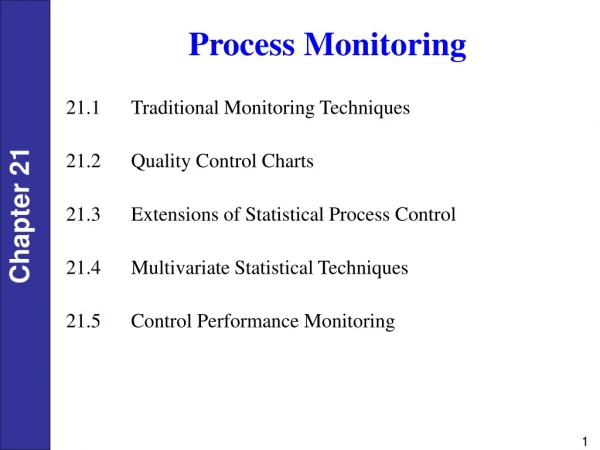
Traditional Monitoring Techniques Limit Checking Process measurements should be checked to ensure that they are between specified limits, a procedure referred to as limit checking. The most common types of measurement limits are: • High and low limits • High limit for the absolute value of the rate of change • Low limit for the sample variance The limits are specified based on safety and environmental considerations, operating objectives, and equipment limitations. • In practice, there are physical limitations on how much a measurement can change between consecutive sampling instances.
Both redundant measurements and conservation equations can be used to good advantage. • A process consisting of two units in a countercurrent flow configuration is shown in Fig. 21.2. • Three steady-state mass balances can be written, one for each unit plus an overall balance around both units. • Although the three balances are not independent, they provide useful information for monitoring purposes. • Industrial processes inevitably exhibit some variability in their manufactured produces regardless of how well the processes are designed and operated. • In statistical process control, an important distinction is made between normal (random) variability and abnormal (nonrandom) variability.
Random variability is caused by the cumulative effects of a number of largely unavoidable phenomena such as electrical measurement noise, turbulence, and random fluctuations in feedstock or catalyst preparation. • The source of this abnormal variability is referred to as a special cause or an assignable cause. Normal Distribution • Because the normal distribution plays a central role in SPC, we briefly review its important characteristics. • The normal distribution is also known as the Gaussian distribution.
Suppose that a random variable x has a normal distribution with a mean and a variance denoted by The probability that x has a value between two arbitrary constants, a and b, is given by where f(x) is the probability density function for the normal distribution: The following probability statements are valid for the normal distribution (Montgomery and Runger, 2003),
Figure 21.3 Probabilities associated with the normal distribution (From Montgomery and Runger (2003)).
For the sake of generality, the tables are expressed in terms of the standard normal distribution, N (0, 1), and the standard normal variable, • It is important to distinguish between the theoretical mean , and the sample mean . • If measurements of a process variable are normally distributed, the sample mean is also normally distributed. • However, for any particular sample, is not necessarily equal to . The Control Chart In statistical process control, Control Charts (or Quality Control Charts) are used to determine whether the process operation is normal or abnormal. The widely used control chart is introduced in the following example.
This type of control chart is often referred to as a Shewhart Chart, in honor of the pioneering statistician, Walter Shewhart, who first developed it in the 1920s. Example 21.1 A manufacturing plant produces 10,000 plastic bottles per day. Because the product is inexpensive and the plant operation is normally satisfactory, it is not economically feasible to inspect every bottle. Instead, a sample of n bottles is randomly selected and inspected each day. These n items are called a subgroup, and n is referred to as the subgroup size. The inspection includes measuring the toughness of x of each bottle in the subgroup and calculating the sample mean
The control chart in Fig. 21.4 displays data for a 30-day period. The control chart has a target (T), an upper control limit (UCL), and a lower control limit (LCL). The target (or centerline) is the desired (or expected) value for , while the region between UCL and LCL defines the range of normal variability, as discussed below. If all of the data are within the control limits, the process operation is considered to be normal or “in a state of control”. Data points outside the control limits are considered to be abnormal, indicating that the process operation is out of control. This situation occurs for the twenty-first sample. A single measurement located slightly beyond a control limit is not necessarily a cause for concern. But frequent or large chart violations should be investigated to determine a special cause.
Control Chart Development • The first step in devising a control chart is to select a set of representative data for a period of time when the process operation is believed to be normal, that is, when the process is in a state of control. • Suppose that these test data consist of N subgroups that have been collected on a regular basis (for example, hourly or daily) and that each subgroup consists of n randomly selected items. • Let xij denote the jth measurement in the ith subgroup. Then, the subgroup sample means can be calculated: (i = 1,2,…, N)
The grand mean is defined to be the average of the subgroup means: The general expressions for the control limits are where is an estimate of the standard deviation for and c is a positive integer; typically, c = 3. • The choice of c = 3 and Eq. 21-6 imply that the measurements will lie within the control chart limits 99.73% of the time, for normal process operation. • The target T is usually specified to be either or the desired value of
The estimated standard deviation can be calculated from the subgroups in the test data by two methods: (1) the standard deviation approach, and (2) the range approach (Montgomery and Runger, 2003). • By definition, the rangeR is the difference between the maximum and minimum values. • Consequently, we will only consider the standard deviation approach. The average sample standard deviation for the N subgroups is:
where the standard deviation for the ith subgroup is If the x data are normally distributed, then is related to by where c4 is a constant that depends on n and is tabulated in Table 21.1.
The s Control Chart • In addition to monitoring average process performance, it is also advantageous to monitor process variability. • The variability within a subgroup can be characterized by its range, standard deviation, or sample variance. • Control charts can be developed for all three statistics but our discussion will be limited to the control chart for the standard deviation, the s control chart. • The centerline for the s chart is , which is the average standard deviation for the test set of data. The control limits are Constants B3 and B4 depend on the subgroup size n, as shown in Table 21.1.
Example 21.2 In semiconductor processing, the photolithography process is used to transfer the circuit design to silicon wafers. In the first step of the process, a specified amount of a polymer solution, photoresist, is applied to a wafer as it spins at high speed on a turntable. The resulting photoresist thickness x is a key process variable. Thickness data for 25 subgroups are shown in Table 21.2. Each subgroup consists of three randomly selected wafers. Construct and s control charts for these test data and critcially evaluate the results. Solution The following sample statistics can be calculated from the data in Table 21.2: = 199.8 Å, = 10.4 Å. For n = 3 the required constants from Table 21.1 are c4 = 0.8862, B3 = 0, and B4 = 2.568. Then the and s control limits can be calculated from Eqs. 21-9 to 21-15.
The traditional value of c = 3 is selected for Eqs. (21-9) and (21-10). The resulting control limits are labeled as the “original limits” in Fig. 21.5. Figure 21.5 indicates that sample #5 lies beyond both the UCL for both the and s control charts, while sample #15 is very close to a control limit on each chart. Thus, the question arises whether these two samples are “outliers” that should be omitted from the analysis. Table 21.2 indicates that sample #5 includes a very large value (260.0), while sample #15 includes a very small value (150.0). However, unusually large or small numerical values by themselves do not justify discarding samples; further investigation is required. Suppose that a more detailed evaluation has discovered a specific reason as to why measurements #5 and #15 should be discarded (e.g., faulty sensor, data misreported, etc.). In this situation, these two samples should be removed and control limits should be recalculated based on the remaining 23 samples.
These modified control limits are tabulated below as well as in Fig. 21.5.
Theoretical Basis for Quality Control Charts The traditional SPC methodology is based on the assumption that the natural variability for “in control” conditions can be characterized by random variations around a constant average value, where x(k) is the measurement at time k, x* is the true (but unknown) value, and e(k) is an additive error. Traditional control charts are based on the following assumptions: • Each additive error, {e(k), k = 1, 2, …}, is a zero mean, random variable that has the same normal distribution, • The additive errors are statistically independent and thus uncorrelated. Consequently, e(k) does not depend on e(j) for j≠ k.
The true value of x* is constant. • The subgroup size n is the same for all of the subgroups. The second assumption is referred to as the independent, identically, distributed (IID) assumption. Consider an individuals control chart for x with x* as its target and “3 control limits”: • These control limits are a special case of Eqs. 21-9 and 21.10 for the idealized situation where is known, c = 3, and the subgroup size is n = 1. • The typical choice of c = 3 can be justified as follows. • Because x is , the probability p that a measurement lies outside the 3 control limits can be calculated from Eq. 21-6: p = 1 – 0.9973 = 0.0027.
Thus on average, approximately 3 out of every 1000 measurements will be outside of the 3 limits. • The average number of samples before a chart violation occurs is referred to as the average run length (ARL). • For the normal (“in control”) process operation, • Thus, a Shewhart chart with 3 control limits will have an average of one control chart violation every 370 samples, even when the process is in a state of control. • Industrial plant measurements are not normally distributed. • However, for large subgroup sizes (n > 25), is approximately normally distributed even if x is not, according to the famous Central Limit Theorem of statistics (Montgomery and Runger, 2003).
Fortunately, modest deviations from “normality” can be tolerated. • In industrial applications, the control chart data are often seriallycorrelated because the current measurement is related to previous measurements. • Standard control charts such as the and s charts can provide misleading results if the data are serially correlated. • But if the degree of correlation is known, the control limits can be adjusted accordingly (Montgomery, 2001). Pattern Tests and the Western Electric Rules • We have considered how abnormal process behavior can be detected by comparing individual measurements with the and s control chart limits. • However, the pattern of measurements can also provide useful information.
A wide variety of pattern tests (also called zone rules) can be developed based on the IID and normal distribution assumptions and the properties of the normal distribution. • For example, the following excerpts from the Western Electric Rules indicate that the process is out of control if one or more of the following conditions occur: • One data point is outside the 3 control limits. • Two out of three consecutive data points are beyond a 2 limit. • Four out of five consecutive data points are beyond a 1 limit and on one side of the center line. • Eight consecutive points are on one side of the center line. • Pattern tests can be used to augment Shewhart charts.
Although Shewhart charts with 3 limits can quickly detect large process changes, they are ineffective for small, sustained process changes (for example, changes smaller than 1.5 ) • Two alternative control charts have been developed to detect small changes: the CUSUM and EWMA control charts. • They also can detect large process changes (for example, 3 shifts), but detection is usually somewhat slower than for Shewhart charts. CUSUM Control Chart • The cumulative sum (CUSUM) is defined to be a running summation of the deviations of the plotted variable from its target. • If the sample mean is plotted, the cumulative sum, C(k), is
where T is the target for . • During normal process operation, C(k) fluctuates around zero. • But if a process change causes a small shift in , C(k) will drift either upward or downward. • The CUSUM control chart was originally developed using a graphical approach based on V-masks. • However, for computer calculations, it is more convenient to use an equivalent algebraic version that consists of two recursive equations, where C+ and C- denote the sums for the high and low directions and K is a constant, the slack parameter.
The CUSUM calculations are initialized by setting C+(0) = C-(0) = 0. • A deviation from the target that is larger than K increases either C+ or C-. • A control limit violation occurs when either C+ or C- exceeds a specified control limit (or threshold), H. • After a limit violation occurs, that sum is reset to zero or to a specified value. • The selection of the threshold H can be based on considerations of average run length. • Suppose that we want to detect whether the sample mean has shifted from the target by a small amount, . • The slack parameter K is usually specified as K = 0.5 .
For the ideal situation where the normally distributed and IID assumptions are valid, ARL values have been tabulated for specified values of , K, and H (Ryan, 2000; Montgomery, 2001). Table 21.3 Average Run Lengths for CUSUM Control Charts
EWMA Control Chart • Information about past measurements can also be included in the control chart calculations by exponentially weighting the data. • This strategy provides the basis for the exponentially-weighted moving-average (EWMA) control chart. • Let denote the sample mean of the measured variable and z denote the EWMA of . A recursive equation is used to calculate z(k), where is a constant, • Note that Eq. 21-27 has the same form as the first-order (or exponential) filter that was introduced in Chapter 17.
The EWMA control chart consists of a plot of z(k) vs. k, as well as a target and upper and lower control limits. • Note that the EWMA control chart reduces to a Shewhart chart for = 1. • The EWMA calculations are initialized by setting z(0) = T. • If the measurements satisfy the IID condition, the EWMA control limits can be derived. • The theoretical limits are given by where is determined from a set of test data taken when the process is in a state of control. • The target T is selected to be either the desired value of or the grand mean for the test data, .
Time-varying control limits can also be derived that provide narrower limits for the first few samples, for applications where early detection is important (Montgomery, 2001; Ryan, 2000). • Tables of ARL values have been developed for the EWMA method, similar to Table 21.3 for the CUSUM method (Ryan, 2000). • The EWMA performance can be adjusted by specifying . • For example, = 0.25 is a reasonable choice because it results in an ARL of 493 for no mean shift ( = 0) and an ARL of 11 for a mean shift of • EWMA control charts can also be constructed for measures of variability such as the range and standard deviation.
Example 21.3 In order to compare Shewhart, CUSUM, and EWMA control charts, consider simulated data for the tensile strength of a phenolic resin. It is assumed that the tensile strength x is normally distributed with a mean of = 70 MPa and a standard deviation of = 3 MPa. A single measurement is available at each sampling instant. A constant was added to x(k) for in order to evaluate each chart’s ability to detect a small process shift. The CUSUM chart was designed using K = 0.5 and H = 5 , while the EWMA parameter was specified as = 0.25. The relative performance of the Shewhart, CUSUM, and EWMA control charts is compared in Fig. 21.6. The Shewhart chart fails to detect the 0.5 shift in x. However, both the CUSUM and EWMA charts quickly detect this change because limit violations occur about ten samples after the shift occurs (at k = 20 and k = 21, respectively). The mean shift can also be detected by applying the Western Electric Rules in the previous section.
Figure 21.6 Comparison of Shewhart (top), CUSUM (middle), and EWMA (bottom) control charts for Example 21.3.
Process Capability Indices • Process capability indices (or process capability ratios) provide a measure of whether an “in control” process is meeting its product specifications. • Suppose that a quality variable x must have a volume between an upper specification limit (USL) and a lower specification limit (LSL), in order for product to satisfy customer requirements. • The Cpcapability index is defined as, where is the standard deviation of x.
Suppose that Cp = 1 and x is normally distributed. • Based on Eq. 21-6, we would expect that 99.73% of the measurements satisfy the specification limits. • If Cp > 1, the product specifications are satisfied; for Cp < 1, they are not. • A second capability index Cpk is based on average process performance ( ), as well as process variability ( ). It is defined as: • Although both Cp and Cpk are used, we consider Cpk to be superior to Cp for the following reason. • If = T, the process is said to be “centered” and Cpk = Cp. • But for ≠ T, Cp does not change, even though the process performance is worse, while Cpkdecreases. For this reason, Cpk is preferred.
In practical applications, a common objective is to have a capabilityindex of 2.0 while a value greater than 1.5 is considered to be acceptable. • Three important points should be noted concerning the Cp and Cpk capability indices: • The data used in the calculations do not have to be normally distributed. • The specification limits, USL and LSL, and the control limits, UCL and LCL, are not related. The specification limits denote the desired process performance, while the control limits represent actual performance during normal operation when the process is in control.
The numerical values of the Cp and Cpk capability indices in (21-25) and (21-26) are only meaningful when the process is in a state of control. However, other process performance indices are available to characterize process performance when the process is not in a state of control. They can be used to evaluate the incentives for improved process control (Shunta, 1995). Example 21.4 Calculate the average values of the Cp and Cpkcapability indices for the photolithography thickness data in Example 21.2. Omit the two outliers (samples #5 and #15) and assume that the upper and lower specification limits for the photoresist thickness are USL=235 Å and LSL = 185 Å.
Solution After samples #5 and #15 are omitted, the grand mean is Å, and the standard deviation of (estimated from Eq. (21-13) with c4 = 0.8862) is Å From Eqs. 21-25 and 21-26, Note the Cpk is much smaller than the Cp because is closer to the LSL than the USL.
Six Sigma Approach • Product quality specifications continue to become more stringent as a result of market demands and intense worldwide competition. • Meeting quality requirements is especially difficult for products that consist of a very large number of components and for manufacturing processes that consist of hundreds of individual steps. • For example, the production of a microelectronics device typically requires 100-300 batch processing steps. • Suppose that there are 200 steps and that each one must meet a quality specification in order for the final product to function properly. • If each step is independent of the others and has a 99% success rate, the overall yield of satisfactory product is (0.99)200 =0.134 or only 13.4%.
Six Sigma Approach • This low yield is clearly unsatisfactory. • Similarly, even when a processing step meets 3 specifications (99.73% success rate), it will still result in an average of 2700 “defects” for every million produced. • Furthermore, the overall yield for this 200-step process is still only 58.2%. • Suppose that a product quality variable x is normally distributed, • As indicated on the left portion of Fig. 21.7, if the product specifications are , the product will meet the specifications 99.999998% of the time. • Thus, on average, there will only be two defective products for every billion produced.
Now suppose that the process operation changes so that the mean value is shifted from to either or , as shown on the right side of Fig. 21.7. • Then the product specifications will still be satisfied 99.99966% of the time, which corresponds to 3.4 defective products per million produced. • In summary, if the variability of a manufacturing operation is so small that the product specification limits are equal to , then the limits can be satisfied even if the mean value of x shifts by as much as 1.5 • This very desirable situation of near perfect product quality is referred to as six sigma quality.
Figure 21.7 The Six Sigma Concept (Montgomery and Runger, 2003). Left: No shift in the mean. Right: 1.5 shift.
Comparison of Statistical Process Control and Automatic Process Control • Statistical process control and automatic process control (APC) are complementary techniques that were developed for different types of problems. • APC is widely used in the process industries because no information is required about the source and type of process disturbances. • APC is most effective when the measurement sampling period is relatively short compared to the process settling time and when the process disturbances tend to be deterministic (that is, when they have a sustained nature such as a step or ramp disturbance). • In statistical process control, the objective is to decide whether the process is behaving normally and to identify a special cause when it is not.
In contrast to APC, no corrective action is taken when the measurements are within the control chart limits. • From an engineering perspective, SPC is viewed as a monitoring rather than a control strategy. • It is very effective when the normal process operation can be characterized by random fluctuations around a mean value. • SPC is an appropriate choice for monitoring problems where the sampling period is long compared to the process settling time, and the process disturbances tend to be random rather than deterministic. • SPC has been widely used for quality control in both discrete- parts manufacturing and the process industries. • In summary, SPC and APC should be regarded as complementary rather than competitive techniques.
They were developed for different types of situations and have been successfully used in the process industries. • Furthermore, a combination of the two methods can be very effective. Multivariate Statistical Techniques • For common SPC monitoring problems, two or more quality variables are important, and they can be highly correlated. • For example, ten or more quality variables are typically measured for synthetic fibers. • For these situations, multivariable SPC techniques can offer significant advantages over the single-variable methods discussed in Section 21.2. • In the statistics literature, these techniques are referred to as multivariate methods, while the standard Shewhart and CUSUM control charts are examples of univariate methods.
Example 21.5 The effluent stream from a wastewater treatment process is monitored to make sure that two process variables, the biological oxidation demand (BOD) and the solids content, meet specifications. Representative data are shown in Table 21.4. Shewhart charts for the sample means are shown in parts (a) and (b) of Fig. 21.8. These univariate control charts indicate that the process appears to be in-control because no chart violations occur for either variable. However, the bivariate control chart in Fig. 21.8c indicates that the two variables are highly correlated because the solids content tends to be large when the BOD is large and vice versa. When the two variables are considered together, their joint confidence limit (for example, at the 99% confidence level) is an ellipse, as shown in Fig. 21.8c. Sample # 8 lies well beyond the 99% limit, indicating an out-of-control condition.