Download
1 / 86
870 likes | 1.02k Vues
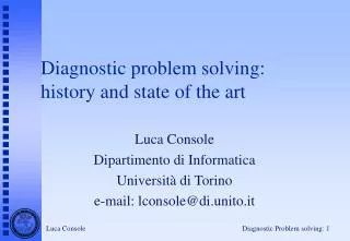
Diagnostic problem solving: history and state of the art. Luca Console Dipartimento di Informatica Università di Torino e-mail: lconsole@di.unito.it. Summary. Introduction to diagnostic problem solving The ‘70s: heuristic approaches to diagnosis The ‘80s critique to the heuristic approach

E N D
Diagnostic problem solving:history and state of the art Luca Console Dipartimento di Informatica Università di Torino e-mail: lconsole@di.unito.it
Summary • Introduction to diagnostic problem solving • The ‘70s: heuristic approaches to diagnosis • The ‘80s • critique to the heuristic approach • model-based diagnosis: the beginnings and the basic techniques • The ‘90s: state of the art • The ‘00: opportunities for the future
Diagnostic Problem Solving • A definition:: diagnosis = finding malfunctions (faults, diseases ...) in a system starting from a set of observations (measurements, tests, symptoms, examinations ...) • A fundamental area for AI from the ‘70s: • Many AI methodologies originated from diagnosis and then spred to other areas of AI • An area of experimentation of different ideas and techniques • A meeting point for many methodologies • A blend of theoretical and experimental research
The ‘70s: heuristic diagnosis • the ‘70s: the expert systems age diagnosis is one of the main experimentation areas for expert systems • a well-defined problem with definite boundaries • specific domain knowledge to be represented • specific reasoning and problem solving strategies • Basic assumptions: diagnosis = heuristic process • experts rely on associational knowledge of the form symptoms faults (diseases) • knowledge derives from experience • knowledge can be elicited from domain experts and represented using suitable KR languages
domain heuristic - associational expert knowledge Heuristic match data abstractions solution abstractions Data Refinement abstraction data solutions (observations) diagnosis = heuristic classification “heuristic classification” [Clancey, 85] “hierarchical classification” [Chandrasekaran, 83]
domain expert (and knowledge engineer) K.A. interface inference K.B engine control K.B. work. mem. user interface final user Diagnostic expert systems: conceptual view
Diagnostic expert systems (II) • many different implementation of the conceptual scheme • E.g.: heuristic 8associational) knowledge represented using • production rules • frames • hybrid formalisms integrating rules and frames Many of these formalisms originated from diagnosis (the use of rules, integrating frames and rules...) • many different applications • medicine, industrial processes, mechanics, aereonautics, ...
Case study 1: Mycin [Stanford Univ. 72-79] • Diagnosis and therapy of bacterial infections • Knowledge base: production rules (original proposal) if (1) the stain of the organism is gram-negative (2) the morphology of the organisms is coccus (3) the growth configuration of the organism is chains then there is a suggestive evidence (0.7) that the identity of the organisms is streptococcus • Inference strategy: backward chaining • Approximate reasoning: ad-hoc heuristic approach • Explanations: HOW, WHY, WHY-NOT ... • Meta-rules for control • from Mycin to Emycin and many other applications
Case study 2: DELTA-CATS1 [General Electric] • Diagnosis and repair of diesel locomotives • goal: support the technicians’ work • Knowledge representation: production rules with forward chaining • Sophisticated approach to uncertain reasoning • graphical interface for providing explanations on drawings of the devices; the repair sequences (stored on the disk) are shown to the technician • [Bonissone et al. 84]
Case study 3: PIP [MIT, 72-78] • Diagnosis of spleen diseases • Knowledge base: stereotypical descriptions based on frames Triggers: <set of symptoms used to evoke the hypothesis> Decision Criteria is-sufficient: < set of symptoms > must-have: < set of symptoms > must-not-have: < set of symptoms > Complementary relation to other diseases caused-by: <set of diseases> cause-of: < set of diseases > complicated-by: < set of diseases > complication-of: < set of diseases > associated-with: < set of diseases > Competing Hypotheses alternative-to: < set of diseases > Score evaluation functions • Inference: • triggering, match and depending on the degree of match, activation of associated or alternative hypotheses • from PIP to a shell and to other applications
Case study 4: hierarchical classification • many systems: Internist/Caduceous/QMR [CMU, 77 ...], MDX [Ohio State, 81-85] LITO [Torino, 79-86] • Hierarchy of diagnostic hypotheses (specialists) • Each specialists: frame and rules • Hierarchical visit based on match and specialization • Experiences are fundamental for many expert system shells of the ‘80s (e.g. KEE/kappa, Nexpert Object, CLIPS ...) • Example: Internist/QMR Internal Medicine ...... Lung diseases Liver diseases .... tumours cirrhosis hepatitis ...........
A summary of the approach: diagnosis of devices • Physical device to be diagnosed (e.g. electronic device) • Heuristic knowledge elicited from a domain expert: associtions • symptoms faults • rules: if inpi1=x1 and ... and inpik= xk and outj1=Y1 • and ... and outjl=Yl then (0.75) fault=P • stereotypical descriptions • fault P: trigger: outjm=ym • symptoms: necessary ( ...) sufficient (....) ...
Critiques to the heuristic approach • The heuristic approach allows one to build diagnostic systems suitable for many problems and applications • well consolidated approach • many tools available • many validated applications in use • Some serious problems • difficulties in acquiring and maintaining the knowledge base • experience knowledge • it is not easy to find experts who are usually not available • subjective knowledge dependent on the specific expert • how to diagnose “new” devices? • how to deal with “new” cases?
Critiques to the heuristic approach (II) • some serious problems (contd) • approach based on classification • it is impossible to deal with cases not considered a-priori • it is difficult to deal with multiple faults • brittleness • Knowledge base specific for diagnosis and not reusable in other tasks • lack of generality and strict dependence on the specific device • it is impossible to reuse knowledge in similar devices or even in new versions of the same device • limited explanation capabilities
The ‘80s: model-based reasoning • New tendency (late 70s - beginning of the 80’s) experience heuristic knowledge model of the system to be diagnosed • “objective” model, not specific for diagnosis (task independent) • New approach to knowledge-based systems • based on “deep knowledge” • based on “first principles” • second-generation expert systems • “model-based”
.... design textbook first principles actual system model of the system observed behaviour predicted behaviour diagnosis Model-based diagnosis • “knowledge level” view: • Different approaches • different types of models • different definitions of diagnosis
Genesis of the model-based approach • Two different evolutions • Diagnosis on causal models • “process centered” approach • born in medical domains, then application to diagnosis of industrial processes and devices • model: causal description of the behavior of the system, in normal and/or faulty conditions • Diagnosis on models of structure and function • “component centered” approach • born in technical domains, then other applications • model: description of the structure of a device (components and their connections) and of the function of each type of component
Diagnosis on causal models • Born in medical applications from the need of modeling physiological and pathophysiological processes for • avoid knowledge which is too heuristic and based on experience • being able to provide causal explanations • need of separating different types of knowledge that are often mixed in the heuristic approach (e.g., domain and control knowledge) • Casnet [Weiss, Kulikowski, 78], ABEL [Patil, 81], SC [Reggia, 83] HEART_FAILURE [Long, 83], CHECK [Console, Torasso, 86] MDX-II [Chandrasekaran, Sticklen, 87] • Similar techniques also in other domains, • mechanics: IDM [Fink et al. 85], DIVA [David et al. 88] CHECK [Console, Torasso, 87] • industrial processes: IDS [Pan, 84] • geology, GTD [Simmons, 88]
causal models of the behaviour (correct and/or faulty) diagnosis = covering (explanation) of the observations via causal chains originated by the faulty behaviour Diagnosis on causal models (II) .... design textbook first principles actual model system of the system observed predicted behaviour behaviour diagnosis
oil_cup radiator normal holed normal holed oil_loss oil_level water_level oil_below_car normal low normal low oil_gauge water_temp normal red normal high engine_on normal high engine_temp A simple example Model: oil_cup(normal) oil_level(normal) oil_cup(holed) oil_loss(present) oil_loss(present) oil_below_car(present) oill_loss(present) oil_level(low) oil_level(normal) oil_gauge(normal) oil_level(low) oil_gauge(red) oil_level(normal) water_level(normal) engine(on) engine_temp(normal) oil_level(low) engine(on) engine_temp(high) ...
Defining and computing diagnoses • Diagnosis: • Given a set of observations • determine a (minimal) set of faults whose consequences cover the observations • “Knowledge level”: diagnosis = abductive process • determine an explanation of the observations using the model as the domain theory • Abduction: • Given a theory T and a set Obs of observations to be explained • Determine a set E such that • T E |= Obs • T E consistent • Diagnosis as set covering
oil_cup radiator normal holed normal holed oil_loss oil_level water_level oil_below_car normal low normal low oil_gauge water_temp normal red normal high engine_on normal high engine_temp Example • Obs1 = {engine_temp(high)} Two minimal candidate explanations • E1 = { oil_cup(holed) } • E2 = {radiator(holed)}
oil_cup radiator normal holed normal holed oil_loss oil_level water_level oil_below_car normal low normal low oil_gauge water_temp normal red normal high engine_on normal high engine_temp Example • Obs2 = {oil_gauge(red), engine_temp(high)} One minimal candidate explanation • E1 = { oil_cup(holed) }
oil_cup radiator normal holed normal holed oil_loss oil_level water_level oil_below_car normal low normal low oil_gauge water_temp normal red normal high engine_on normal high engine_temp Example • Obs3 = {oil_gauge(red), water_temperature(high)} One minimal candidate explanation • E1 = { oil_cup(holed), radiator(holed)}
Diagnosis on models of structure and function • Originated in technical domains (hardware diagnosis) from • difficulties in gaining experience with devices (short life cycle) • need of diagnosing “new” devices” • need of reusing models • Three main projects at the beginning of the ‘80s • Sophie (MIT U. Cal Irvine, BBN, poi XeroX) • seminal paper “How Circuit works“ [deKleer, 76] • tutoring system for HW diagnosis • HT project at MIT [Davis, 83, 84] • models of structure and function, reasoning techniques • DART project at Stanford [Genesereth, 84] • logical languages for modeling for diagnosis and design • Application to other domains
diagnosis = removing discrepancies between the nominal predicted behaviour and the observed one Diagnosis on models of structure and function(II) .... design textbook first principles actual model device of the device observed predicted model of the structure behaviour behaviour of the device and of the (nominal) behaviour of each type of component diagnosi
2 Mult1 3 Add1 A 2 Mult2 3 Add2 B 2 Mult3 3 A simple (classical) example Model Function of each type of component: Adder(X) not AB(X) out(X) = inp1(X) + inp2(X) Multiplier(X) not AB(X) out(X) = inp1(X) * inp2(X) ... Structure (functional structure): Multiplier(Mult1), Multiplier(Mult2), Multiplier(Mult3), Adder(Add1), Adder(Add2) out(Mult1) = inp1(Add1) out(Mult2) = inp2(Add1) = inp1(Add2) out(Mult3) = inp2(Add2)
Defining and computing diagnoses • Generating prediction starting from the model of the correct behaviour (and the inputs) • Analysis of the discrepancies between predicted and observed behaviour; for each predicted value that differs from the observed one: • conflict = set of components involved in the discrepancy; they cannot be all working properly • generating all conflicts (actually only the minimal ones) • at least one component in each conflict must be faulty
2 Mult1 3 Add1 A 2 Mult2 3 Add2 B 2 Mult3 3 Example Prediction: A=12, B=12 Observation A=10, B=12 • A=10 generates two conflicts: • {Add1, Mult1, Mult2} • {Add1, Mult1, Mult3, Add2} 12 10 12 12
Defining and computing diagnoses (contd.) • Generating prediction starting from the model of the correct behaviour (and the inputs) • Analysis of the discrepancies between predicted and observed behaviour; for each predicted value that differs from the observed one: • conflict = set of components involved in the discrepancy; they cannot be all working properly • generating all conflicts (actually only the minimal ones) • at least one component in each conflict must be faulty • Generating diagnoses from conflicts • diagnosis = (minimal) hitting set of the conflicts • intersection between the conflicts provides single-fault diagnoses
2 Mult1 3 Add1 A 2 Mult2 3 Add2 B 2 Mult3 3 Esempio Prediction: A=12, B=12 Observation A=10, B=12 • A=10 generates two conflicts: • {Add1, Mult1, Mult2} • {Add1, Mult1, Mult3, Add2} 10 • Candidates (minimal hitting sets) • single faults {Add1} {Mult1} • double faults {Mult2, Mult3}, • {Add2, Mult2} 12
Defining and computing diagnoses (contd.) • Generating prediction starting from the model of the correct behaviour (and the inputs) • Analysis of the discrepancies between predicted and observed behaviour; for each predicted value that differs from the observed one: • conflict = set of components involved in the discrepancy; they cannot be all working properly • generating all conflicts (actually only the minimal ones) • at least one component in each conflict must be faulty • Generating diagnoses from conflicts • diagnosis = (minimal) hitting set of the conflicts • intersection between the conflicts provides single-fault diagnoses • (optional) corroboration principle • exonerate all the components involved in each concordance between observed and predicted behavior,
2 Mult1 3 Add1 A 2 Mult2 3 Add2 B 2 Mult3 3 • Applying cooroboration from B=12 • exonerate Add2, Mult2, Mult3 • candidates: {Add1}, {Mult1} Esempio Prediction: A=12, B=12 Observation A=10, B=12 • A=10 generates two conflicts: • {Add1, Mult1, Mult2} • {Add1, Mult1, Mult3, Add2} 10 • Candidates (minimal hitting sets) • single faults {Add1} {Mult1} • double faults {Mult2, Mult3}, • {Add2, Mult2} 12
Defining and computing diagnoses (II) • use of the Assumption Based Truth Maintenance System (ATMS) for computing diagnoses • “Knowledge level”: diagnosis = form of default reasoning • default: each component behaves normal, if this is consistent: • diagnoses: extensions of a default theory whose logical theory is the models and whose defaults are as above [Reiter, 87] • Consistency-based diagnosis
Exploiting models of correct/faulty behaviour • Goal of model-based diagnosis: using models that are • easy to acquire • reusable • for diagnosing different devices (having the same components) • for different tasks (e.g. simulation, FMEA, ..) • Initial proposal: using only models of correct behaviour • They are those that are in strict accordance with the goals • but unfortunately they are not always sufficient • need of exploiting also fault models of some form • predictive models [Struss, Dressle, 89] [de Kleer, Williams 89] • “weak” models of physical impossibility [Friedrich et al. 90] • behavioural models [Console, Torasso, 91]
Observations: light(B-1,off), light( B-2,off), light( B-3,ok) Example Model of the correct behaviour battery(S) not AB(S) voltageOut(S,ok) bulb(B) not AB(B) voltageIn(B,X) light(B,X) wire(W) not AB(B) voltageIn(W,X) voltageOut(W,X) • Candidates: • {B-1, B-2}, • {S, B-3}, {S, W-3}, {W1, W3} ..... NONSENSE!!!!! • Fault models are needed • predictive: bulb(B) AB(B) voltageIn(B,X) light(B,off) • weak: “physical impossibility” : not(AB(W) and voltageOut(W,ok)
Diagnosis on behavioural models: a spectrum of definitions • behavioural models [deKleer, Williams, 89]: • set of modes of behaviour for each component • set of constraints (rules) for each mode • Definition of diagnosis [ Console, Torasso, 91]: • integrating abductive and consistency-based diagnosis • abduction and consistency are the two extremes of a spectrum of alternatives • abduction is the most restrictive definition • it requires “complete” models • it provides a strong (physical) notion of explanation • consistency-based is less restrictive • less constraints on the models • weaker notion of explanation
Diagnosis on behavioural models: a spectrum of definitions (II) abduction consistency-based • Criteria for comparing the alternatives • Criteria for choosing the “right” definition, given the available model and observability conditions ordering: set inclusion consistency-based abduction lattice of definitions Lattice of sets of solutions
Diagnosis as a process generation of the candidates from initial observations • Diagnosi s is an iterative process • Different halting conditions for different goals: • fault detection • fault localization • fault identification • Overall goal: repair the system, not only diagnose it Yes Stop? No generates - probe - test for disrimination update candidates
Generation of tests/probes • based on • predictions generated by each candidate on unknown measurable points • cost/risk/benefits of the different tests/probes • fault proability of the various components • Approach based on entropy [deKleer, 87, 92] • a-priori probability of the faults (even a rough estimate) • given set D1, D2, ... Dn of candidates to be discriminated • generate predictions from each candidate • for each probe/test, compute the a-posteriori probability p(Di|T(x)), for each possible outcome x of T • select the test/probe for which the distribution p(Di|T(x)) has a minimal entropy (this is the test that on average best discriminates between the candidates)
Example • Two candidates D1 e D2 with the same a-priori probability • Two probes (tests) are possible • A with possible values 0 e 1 • B with possible values 0 e 1 • Prediction: • D1 predicts A(0) e B(1) • D2 predicts A(1) e B(1) • Discrimination: • P(D1 | A(0)) = 1, P(D2 | A(0) =0, P(D1 | A(1)) = 0, P(D2 | A(1) =1 • P(D1 | B(0)) = 0, P(D2 | B(0) =0, P(D1 | B(1)) = .5, P(D2 | B(1) =.5 • Then A is the test that on average best discriminates (whatever is the outcome, only one candidate remains)
2 Mult1 3 Add1 A 2 Mult2 3 Measurement Add2 B 2 Mult3 3 Example • Candidates • single faults {Add1} {Mult1}
Integrating diagnosis and repair • Diagnosis is not the final goal: the goal is to repair the system • Defining repair strategies • replacement of components • reconfiguring the system • taking into account the cost of the system breakdown, real time constraints • ... • Integrating diagnosis and repair planning • repair strategies define criteria for halting the diagnosis loop (e.g. it is useless to discriminate between faults that are repaired in the same way) • In some cases it is better to perform a repair action before a complete discrimination between the candidates • opportunistic reasoning strategies
Observation: no power in t2 (house) and in t3(hospital) • candidates: {I1}, {I2} • immediate reconfiguration action: switch breaker b to serve t3 • then discrimination between the candidates (measuring power in t1) and repair - - t3 Example • Power distribution Network (Siemens Austria, Friedrich et al.) t5 t4 t2 b l4 l3 ~ g1 l2 g2 ~ t1 l1
Models of real devices • Modeling is the critical aspect of model-based diagnosis • Each model is an abstraction of the actual physical system • different choices and assumption in modeling • different dimensions (aspects) are captured by different types of models • choosing the models depend on many factors • which pieces of information are available • which are the goals of diagnosis • which observations (and in which form) can be available • which repair and test action can be made • temporal constraints on the behavior of the device and on the diagnostic process • .... • Different dimensions in modeling
Dimensions in modeling (not exhaustive !) process oriented component oriented causal models process models structural models functional models behavioural models teleological models (similar to comp. oriented.) ... ... ... ... crisp probabilistic correct behaviour fault models .... intensional extensional time- varying quantitative qualitative static dynamic hierarchical flat discrete state change landmarks orders of magnitude ... derivatives intervals
Multiple models • Usually combining different types of models (multi-modeling) is a good choice • each type of models captures some aspects and some types of faults “pathways of interaction” [Davis, 84] • Example: electronic (electric) circuit • Model of structure (functional) and function (see above) • captures faults to components • pathways of interaction: input-output behaviour of the components • Model of the physical structure (layout) • captures layout faults (e.g. bridge faults) • pathways of interaction: adjacency of components • teleological model • capture faults in design or in the construction of the device
Analysis of some modeling techniques • Many techniques in use in real systems • Analysis of some of the dimensions listed before • qualitative models • landmarks e qualitative constraints • orders of magnitude • models based on deviations • temporal, dynamic and time-varying models • hierarchical models • probabilistic models
Qualitative models • Quantitative models: • difficult to build (especially for fault models) • usually they are not those on which experts rely for the analysis of a device (of its behaviour, e.g. for diagnosis) • in many cases imprecise knowledge makes numerical models useless (e.g. model of the combustion in an engine) • usually imprecision in the observations • Goal: building models that describe in a qualitative way the behavior of a physical system • many approaches to qualitative reasoning • a research area with very strong connections with model-based diagnosis
Qualitative reasoning • Many AI applications need models of real physical systems • Example: • models of devices for simulations, diagnosis, monitoring, … • models of processes for simulation, monitoring, … • Different types of models can be used • Quantitative (numeric) models: based on mathematical equations • in some cases they are derived from physical laws • but usually • they are difficult to use • they are not what people use to solve problems • Qualitative models • abstract models • they need a “new mathematics”, that is “common-sense” forms of reasoning to solve qualitative equations • closer than numeric models to the way we reason • problem: being more abstract they are less accurate and can be ambiguous