Quantum Information
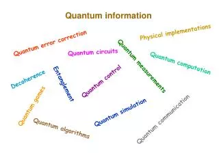
Quantum Information. Stephen M. Barnett University of Strathclyde steve@phys.strath.ac.uk. The Wolfson Foundation. Probability and Information 2. Elements of Quantum Theory 3. Quantum Cryptography 4. Generalized Measurements Entanglement Quantum Information Processing

Quantum Information
E N D
Presentation Transcript
Quantum Information Stephen M. Barnett University of Strathclyde steve@phys.strath.ac.uk The Wolfson Foundation
Probability and Information • 2. Elements of Quantum Theory • 3. Quantum Cryptography • 4. Generalized Measurements • Entanglement • Quantum Information Processing • 7. Quantum Computation • 8. Quantum Information Theory 4.1 Ideal von Neumann measurements 4.2 Non-ideal measurements 4.3 Probability operator measures 4.4 Optimised measurements 4.5 Operations
‘Black box’ 4.1 Ideal von Neumann measurements Measurement model What are the probabilities for the measurement outcomes? How does the measurement change the quantum state?
von Neumann measurements Mathematical Foundations of Quantum Mechanics
(i) An observable A is represented by an Hermitian operator: (ii) A measurement of A will give one of its eigenvalues as a result. The probabilities are or (iii) Immediately following the measurement, the system is left in the associated eigenstate:
More generally for observables with degenerate spectra: (i’) Let be the projector onto eigenstates with eigenvalue : (ii’) The probability that the measurement will give the result is (iii’) The state following the measurement is
a b Detector
Properties of projectors I. They are Hemitian Observable II. They are positive Probabilities III. They are complete Probabilities IV. They are orthonormal ??
‘Black box’ ‘Black box’ 4.2 Non-ideal measurements Real measurements are ‘noisy’ and this leads to errors
We can write these in the form where we have introduced the probability operators For a more general state:
These probability operators are I. Hermitian II. positive III. complete But IV. they are not orthonormal We seem to need a generalised description of measurements
4.3 Probability operator measures Our generalised formula for measurement probabilities is The set probability operators describing a measurement is called a probability operator measure (POM) or a positive operator-valued measure (POVM). The probability operators can be defined by the properties that they satisfy:
Properties of probability operators I. They are Hermitian Observable II. They are positive Probabilities III. They are complete Probabilities IV. Orthonormal ??
S A S + A A S Generalised measurements as comparisons Prepare an ancillary system in a known state: Perform a selected unitary transformation to couple the system and ancilla: Perform a von Neumann measurement on both the system and ancilla:
POM rules: I. Hermiticity: II. Positivity: III. Completeness follows from: The probability for outcome i is The probability operators act only on the system state-space.
Generalised measurements as comparisons We can rewrite the detection probability as is a projector onto correlated (entangled) states of the system and ancilla. The generalised measurement is a von Neumann measurement in which the system and ancilla are compared.
Simultaneous measurement of position and momentum The simultaneous perfect measurement of x and p would violate complementarity. p x Position measurement gives no momentum information and depends on the position probability distribution.
Simultaneous measurement of position and momentum The simultaneous perfect measurement of x and p would violate complementarity. p x Momentum measurement gives no position information and depends on the momentum probability distribution.
Simultaneous measurement of position and momentum The simultaneous perfect measurement of x and p would violate complementarity. p x Joint position and measurement gives partial information on both the position and the momentum. Position-momentum minimum uncertainty state.
Probability density: POM description of joint measurements Minimum uncertainty states:
The associated position probability distribution is This leads us to the POM elements: Increased uncertainty is the price we pay for measuring x and p.
Preparation device Measurement device i selected. prob. Measurement result j Bob is more interested in The communications problem ‘Alice’ prepares a quantum system in one of a set of N possible signal states and sends it to ‘Bob’
In general, signal states will be non-orthogonal. No measurement can distinguish perfectly between such states. Were it possible then there would exist a POM with Completeness, positivity and What is the best we can do? Depends on what we mean by ‘best’.
Minimum-error discrimination We can associate each measurement operator with a signal state . This leads to an error probability Any POM that satisfies the conditions will minimise the probability of error.
For just two states, we require a von Neumann measurement with projectors onto the eigenstates of with positive (1) and negative (2) eigenvalues: Consider for example the two pure qubit-states
The minimum error is achieved by measuring in the orthonormal basis spanned by the states and . We associate with and with : The minimum error is the Helstrom bound
P = |a|2 a + b P = |b|2 A single photon only gives one “click” But this is all we need to discriminate between our two states with minimum error.
A more challenging example is the ‘trine ensemble’ of three equiprobable states: It is straightforward to confirm that the minimum-error conditions are satisfied by the three probability operators
Simple example - the trine states Three symmetric states of photon polarisation
Polarisation interferometer - Sasaki et al, Clarke et al. PBS PBS PBS
Unambiguous discrimination The existence of a minimum error does not mean that error-free or unambiguous state discrimination is impossible. A von Neumann measurement with will give unambiguous identification of : result error-free result inconclusive
Result 1 Result 2 Result ? State 0 State 0 There is a more symmetrical approach with
How can we understand the IDP measurement? Consider an extension into a 3D state-space
Unambiguous state discrimination - Huttner et al, Clarke et al. ? A similar device allows minimum error discrimination for the trine states.
‘Black box’ Measurement model What are the probabilities for the measurement outcomes? How does the measurement change the quantum state?
4.5 Operations How does the state of the system change after a measurement is performed? Problems with von Neumann’s description: 1) Most measurements are more destructive than von Neumann’s ideal. 2) How should we describe the state of the system after a generalised measurement?
Physical and mathematical constraints What is the most general way in which we can change a density operator? Quantum theory is linear so … or more generally BUT this must also be a density operator.
I. They are Hermitian II. They are positive III. They have unit trace The first of these tells us that and this ensures that the second is satisfied. The final condition tells us that Properties of density operators
The operator is positive and this leads us to associate (Knowing does not give us .) If the measurement result is i then the density operator changes as This replaces the von Neumann transformation
If the measurement result is not known then the transformed density operator is the probability-weighted sum which has the form required by linearity. We refer to the operators and as Krauss operators or an an ‘effect’.
Repeated measurements Suppose we perform a first measurement with results i and effect operators and then a second with outcomes j and effects . The probability that the second result is j given that the first was i is
Hence the combined probability operator for the two measurements is If the results i and j are recorded then If they are not known then
Unitary and non-unitary evolution The effects formalism is not restricted to describing measurements, e.g. Schroedinger evolution which has a single Krauss operator . We can also use it to describe dissipative dynamics: Spontaneous decay rate 2g
We can write the evolved density operator in terms of two effects: Measurement interpretation? Has the atom decayed?
State separation Suppose that we have a system known to have been prepared in one of two non-orthgonal states and . Our task is to separate the states, i.e. to transform them into and with so that the states are more orthogonal and hence more distinguishable. This process cannot be guaranteed but can succeed with some probability . How large can this be? Optimal operations: an example What processes are allowed? Those that can be described by effects.
We introduce an effect associated with successful state separation We can bound the success probability by considering the action of on a superposition of the states and noting that the result must be an allowed state:
There is a natural interpretation of this in terms of unambiguous state discrimination: Because this is the maximum allowed, state separation cannot better it so