Download
1 / 41
410 likes | 424 Vues
This text discusses the trigger menu and calibration process for the ATLAS detector, as well as the alignment and stability of the inner detector. It also provides insights into the magnetic field mapping and electron calorimeter calibration.

E N D
I primi 108 trigger in ATLAS Aleandro Nisati, per ATLAS
Some assumptions … • <L> = 1031 cm-2 s-1 ; • Event Filter rate = 100 Hz; (108 events collected) • T = 106 s; • L = 10 pb-1; Not so much for physics…
outline • Trigger menu • Calibrations • Data processing • Computing • Physics more emphasis on italian commitments
Example of a trigger menu (L=6x1031 cm-2 s-1) Physics signatures are selected with cuts that are less stringent than the ones for the “low luminosity” runs. Rates are indicative! • mu6 GeV (2%) 10 Hz • mu 20 GeV 4 Hz • E/gamma 15 GeV 25 Hz • Jet pT> 150 GeV 6 Hz • Missing Energy(40 GeV)+jet 40 GeV 30 Hz • Minimum Bias (prescaled) & Monitor 10 Hz Overall trigger rate: ~90 Hz
ATLAS Detector at the start-up • Stringent construction requirements and quality controls; • Equipped with redundant calibration/alignment hardware systems; • Prototypes and part of final modules extensively tested with test beams (allows also validation of G4 simulation); • Calibration in situ of the detector (accounts for all effects not studied with the test beams) includes: • Test pulses; • Radiactive sources; • Cosmic runs (end 2006—beg 2007); • Beam-halo and beam-gas events during single beam period; What can be done with the first pp data sample ?
Inner Detector • Pixels: 1700 modules, ~100 million cells – middle barrel and disks initially staged • SCT: 4000 modules, 6 million channels • TRT: 370k straws, 420k channels – C wheels initially staged Extremely complex systems – months of commissioning even before ‘physics’ data…
Position accuracy • Individual modules located on supports to 17-100m in r- • Support structures (layers/disks/modules) positioned to 20-200m • X-ray and FSI should reduce these uncertainties for SCT • Whole ID positioned to within 3mm of theoretical beamline • Possible rotation up to 1 mrad wrt beamline, < 1 mrad to solenoid axis • Start system debug and alignment with cosmics and beam-gas interactions
Trackfinding with ‘as installed’ alignment • How well will tracks be found initially ? • Use standard iPatrec trackfinding • Misalign all modules (SCT/pixel) by ‘local’ installation precision (module structure) • Misalign all barrels/disks by RMS 100 m • Reasonable estimate of installed precision • Four examples – different misalignments • Run 10k 6 GeV muons (dc1 002207) • Study track finding efficiency wrt perfect alignment… • 94% efficiency for ‘local’ misalignments • 40-60% efficiency for installed precision • Tracks can still be found (with std cuts) • Should really run with relaxed tolerances • With 500 m RMS, serious degradation • Sometimes very few tracks found • Important to build as precisely as possible
alignment precision estimates - 2 • Calculate r- alignment precision from one day of low luminosity running (here L=1033 cm-2s-1 was assumed): • Use all tracks in modules, or only overlaps (assume 1% - 1.5-3% in DC 1 geometry) • Results given for middle pixel barrel, and 2nd SCT barrel The same is for L=1031 cm-2s-1 in the case of hadrons; scale by sqrt(10) for muons • Statistics to align pixels to 1-2 m and SCT to 2-3 m using 1 day of data taking • Limited by data recording rate rather than luminosity • But systematics will also be important – can make a start with little data
Alignment perspectives • Statistics is not the issue – plenty of data with initial collider running • Plus useful data from cosmics and beam-gas events • Systematics and understanding will be the key issue: • Bringing together the knowledge from survey, tracking and ongoing FSI monitoring • Detector (thermal) stability will become important below 100 mm (initial running conditions will probably be unstable)
Solenoid field mapping • Understanding magnetic field is important for mass scale • W mass requires overall field integral to < 0.05%, other physics processes 0.1% • Shape more difficult – understand local variations to < 0.3%. • Strategy for B-field determination • Mapping field before ID installation using mapping machine with Hall probe array • Intrinsic precision better than 0.1%, measure many points (few days mapping) • Fit field map using Maxwell equations • Field shape can be described to ~ 0.02% using Bessel function expansion • May improve precision by constraining Hall probe measurements • Monitoring using NMR probes during running • 4 NMR probes installed outside barrel TRT at z=0 (region with low field gradient) • Use for checking overall scale and monitoring time stability (probe intrinsic precision of ~ 5 ppm – frequency measurement) • Final check using particles of known masses (J/, , Z) • But this also brings in alignment and material effects – corrections hopefully small
Electromagnetic calorimeter Pb-liquid argon sampling calorimeter with Accordion shape, covering || < 2.5 H : to observe signal peak on top of huge background need mass resolution of ~ 1%response uniformity (i.e. total constant term of energy resolution) 0.7% over || < 2.5
Calorimeter calibration • The constant term c=cL cLR; • The local constant term, cL: • Geometry (residual Accordion modulation) • Mechanics (absorber & gap thickness) • Calibration (with pulse test: amplitude uniformity, etc …) • The “long-range” constant term cLR (from module-to-module miscalibration); • The absolute energy scale Use test beam measurements, cosmic ray run, pp collisions
Scan of a barrel module with 245 GeV e- r.m.s. 0.57% over ~ 500 spots < > = 2.2 mm 9 m • Geometry: (e.g. deviation from Accordion modulation): ~ 0.3%; • Construction phase: thickness of all 1536 absorber plates (1.5m long, 0.5m wide) within ~ 10mm response uniformity <~ 0.3%; • Pulse-Test: calibration accuracy of each module ~ 0.4%; Overall “local” constant term: 0.5-0.6%. • Test-beam: 4 (out of 32) barrel modules and 3 (out of 16) endcap modules; Uniformity over units of size Dh x Df = 0.2x0.4: ~ 0.5%; Test-beam data
Muon signal in barrel ECAL Test-beam data S() / (noise) 7 • Cosmic muons: • find dead/noisy channels; cabling errors; compare with test beam data; • check calibrations; with <3 months of cosmics runs we can correct the calorimeter response variations vs h to 0.5% ; Test-beam data
Beam-halo and beam-gas; • reconstruct muons in the end-cap • rate: ~ 1 Hz for Etot > 5 GeV; open problem: how to trigger? • measure p0 in EM calo and check shower shapes; • Few usable electrons: try to use other tracks to check calibrations • If no correction are applied: • cL ~ 1.3% • cLR~ 1.5% The calorimeter will behave sufficiently well already at the start-up to allow some physics.
With pp collisions • Use min. bias and “some” electron trigger (pT > 10 GeV) • Adjust/set-up timing of calorimeters • Measure “overall” energy spectrum in EM calo • Measure EM cluster energy spectrum • Study response uniformity of calo’s in • Start tuning/adjusting e-identification procedure • Check calo shower shapes for electrons • Combine cluster with tracks • First E/p measurements • Study calo/ID alignment
With pp collisions Try to see first Zee events • Start EM inter-calibration • Calibrate ~400 region ( x = 0.2 x 0.4) • ~ 250 eper region needed to achieve ctot 0.7% • ~ 105 Z ee events needed, ~ 104 Z will be available Likely, c ~ 1% worst case scenario: ctot 2% • cL = 1.3 % measured “on-line” non-uniformity of individual modules • cLR = 1.5 % no calibration with Z ee
Hadronic Calorimeters • Cell calibration: • Reference scale (starting point) for individual cell calibration = EM scale • LAr: testbeam and calibration systems: about 1% accuracy on EM scale • Tilecal: testbeam data, Cs calibration ~ 3.4 % precision on EM scale • Cosmic muons, beam-halo muons • Useful in many aspects • Largon: finding dead channels, cabling errors… • Compare to muon test beam data • Possibility to trigger with Tilecal under study • Beam-gas hadrons • Channel mapping; • Study their properties and how to reject them…
Minimum Bias & jet events • Monitoring detector response stability: with ~ 1-8x10⁶ triggers to reach 1% stability • Cell-to-cell calibration • Using phi-symmetry of MB triggers, inter-calibrate cells with equal dimensions/positions (2x64 cells) • Jet calibration; based on weights estimated from Monte Carlo studies; ingredients: • Jet fragmentation modelling: electromagnetic jet energy fraction, energy and multiplicity of charged hadrons, etc.. • Hadronic shower models, benchmarked in comparison with test beam data; • Description of dead material in simulation (fraction of “lost energy” in dead material from ~few% to 15 %)
Calibration of the L1Calo system up to the start of collisions By using test-pulses the calibration procedures can checked and first Calibration constants can be derived - close to final values Beam-gas collisions (one-beam running) in mid-Detector have the same timing as collision events - the timing setup can derived and checked Test-Pulses Test-Beam signals at known energy ATLAS LAr/Tile Calorimeters L1Calo Trigger Trigger-Inputs Signals from beam- gas collisions Calorimeter Read-out Calibration constants L1Calo Read-out
Calibration of the L1Calo system up to the start of collisions • Important parameters to calibrate: • Timing of input signals and timing inside the system • Transverse momentum / energy calibration • Pedestal values • Pulse shapes • Saturation values • Noise sigma Many other setup parameters needed to ensure correct data-flow in the system - to be determined and checked before collisions start
Calibration of the L1Calo system: The first 108 triggers Calorimeter Expect about 104 Z0 e+e- / 105 W e / … • Clean signals with enough statistics to: • Study the energy calibration • Verify the timing setup and event identification • Map out the threshold curves • Study trigger efficiency Z0 A rapid calibration cycle is needed especially at the beginning.
Muon Detector & Trigger • Preliminary r-t calibration of the MDT tubes; • Calibration of the LVL1 muon trigger system: • System timing; • Coincidence roads; • Evaluation of the single muon trigger efficiency; • Measurement of the cavern background level detected by the muon chambers • Measurement of the muon spectrum and comparison with expectations
Muon Detector & Trigger • MDT calibration • Chamber Alignment • Level-1 Trigger calibration • Detector noise • System synchronization • Trigger efficiency
MDT calibration : to + r/t dn/ dt • ultimate accuracy in to : 0.4 ns • needs ~ 104 hits/tube • O (109) -triggers (geometry + included) to (to) (ns) t(ns) • before pp data : • average to (few × ns) • cosmics during commissioning (sys shift) • cosmics in ATLAS (105 x 100 days 1.5ns) 0.4 ns 104 n
more news soon MDT calibration : to + r/t t(ns) ultimate accuracy in r/t : ~10m needs ~ 2.5×10⁴ good /chamber O (108) -triggers (geometry + included) + temperature+B-field corrections + a lot of computing. r(mm) however, cosmics are seen only in ~ ½ ATLAS use pp data to extend the calibration to full detector, make checks and start final (¿?) pass. • before pp data : • average r/t (100200 m) • cosmics in ATLAS (105/day×100days ok)
Testbeam studies of chamber alignment system reconstructions with nominal geometry show how chambers are misaligned in terms of sagitta and relative angles (barrel, 2nd tower) Mean sagitta = - 0.6 mm
SAGITTA ANALYSIS • 7 BIL2 translations along Z/Rail (16/08/2003), magnet 800A • Analysis with fixed nominalgeometry
SAGITTA ANALYSIS • RUNS WITH BIL2 DISPLACEMENTS, MAGNET 800 A (BL=3.4 Tm) • ANALYSIS WITH ALIGNMENT CORRECTIONS (ASAP) Magnet 800 A Magnet 800 A Mean = -0.59 mm
Alignment system still under test this year in H8; will verify the performance of the overall alignment system: some preliminary result: • The analysis of cosmic ray data will help to further check the initial performance of the optical alignment system. • The pp data will help to check and possibly improve the detector alignment. Conclusion on the alignment accuracy: absolute chamber position within ~ 100-200 mm. Ultimate accuracy: ~ 30 mm;
RPC/TGC counting rate • Intrinsic RPC noise can be measured with LHC off; typical measured noise is about 3 Hz/cm2. • Cavern background (neutron, photons,...): • “Incoherent” physics background: • RPC counting rate: ~0.02 Hz/cm2 physics rate (L=1x1031 cm-2 s-1); • too low wrt detector noise; check that this noise doesn’t depend on LHC on/off; • “Coherent” physics background: count the number of RPC events with the same strip (or +-1) fired in RPC doublets. • Penetrating background particles: specific tools as pattern recognition programs will be used.
Timing of Coincidence Matrices • Pulse test and the run with cosmics will allow a preliminary evaluation of the time alignment of the RPC signal to be put in space and time coincidence; • With pp collisions: can be done with single muons: Assume ~106 muons pT>~10 GeV in the barrel system; => With this statistic we expect about 600 events per Coincidence Matrix (in total 2x1700 CMs), likely sufficient for a first time aligment of each of them. • The trigger system does not need a veryaccurate time alignment when running at low luminosity. • Coincidence Windows: Not a problem. Rely on simulation knowing the collision point position along z with about 1cm accuracy.
Trigger efficiency • Can be done with the study of di-muon systems (J/Y, Z,...) triggered with an inclusive muon selection: analyze the muon with no trigger as a function of h, f and pT.
HPSS HPSS HPSS Northern Tier ~200kSI2k The Computing System ~Pb/sec Event Builder 10 GB/sec Event Filter~1.5MSI2k • Some data for calibration and monitoring to institutes • Calibrations flow back 450 MB/sec Tier 0 T0 ~5MSI2k HPSS ~ 300MB/s/T1 /expt Tier 1 UK Regional Centre (RAL) US Regional Centre Italian Regional Centre French Regional Centre HPSS 622Mb/s Tier 2 Tier2 Centre ~200kSI2k Tier2 Centre ~200kSI2k Tier2 Centre ~200kSI2k 622Mb/s Each Tier 2 has ~25 physicists working on one or more channels Each Tier 2 should have the full AOD, TAG & relevant Physics Group summary data Tier 2 do bulk of simulation Lancaster ~0.25TIPS Liverpool Manchester Sheffield Physics data cache 100 - 1000 MB/s Desktop Workstations
Operation of Tier-0 • The Tier-0 facility at CERN will have to: • Hold a copy of all raw data to tape • Copy all raw data to T-1’s for later reprocessing • Keep calibration data on disk • Store master conditions database here • Run first-pass calibration/alignment and reconstruction • ESD copy retained on tape • Distribute ESD’s to N external Tier-1’s • (2/N to each one of N Tier-1’s; assume N=10 for now) • Express lines • Need for calibration line to reduce latency • Might also serve as physics monitoring line • ‘Physics’ hotline more contentious • Streaming of ESD and AOD • Always envisaged to stream AOD into ~10 exclusive streams, collections being built from unions of streams • Streaming of ESD is required to reduce file access
Operation of Tier-1’s and Tier-2’s Tiers defined by capacity, role and level of service No assumption of single site (esp. T2), but must present as a single entity in human/response terms • We envisage likely10 Tier-1’s for ATLAS. Each one will: • Keep on disk 1/5 of the ESD’s and a full AOD’s and TAG’s • Keep on tape 1/10 of Raw Data, reprocess and retain ESD produced • Keep on disk 1/5 of currently simulated ESD’s and on tape 1/10 of previous versions • Provide facilities for physics group controlled ESD analysis • Calibrations • Support role for defined set of Tier-2s • We estimate ~4 Tier-2’s (various sizes, slower response) for each Tier-1. Each one will: • Keep on disk a full copy of TAG and roughly one full AOD copy per four T2s • Keep on disk a small selected sample of ESD’s • Provide facilities (CPU and disk space) for user analysis and user simulation (~25 users/Tier-2) • Run central simulation
Physics • Study properties of minimum bias events and check with existing data at lower energies. • Study the muon spectrum; check inclusive LVL1 muon trigger rates; • Check: J/Psi, Ypsilon, W and Z to leptons; preliminary estimates of production cross sections of W and Z to leptons, with an expected error of ~ 15-20% (10% lumi;10-15% efficiency) • Inclusive jet cross section measurement • Top signal visible?
Conclusions The first pp events have many invaluable tasks: • Subdetectors: • Calibrations, almost always not final, but improved wrt test-beam and cosmics run • From subdetectors to ATLAS: • Trigger commissioning + efficiency • Subdetector integration and event building • Offline commissioning • From detector to results: • Some very preliminary physics analysis: W, Z cross-sections, jet spectrum, …