Download
1 / 52
520 likes | 727 Vues
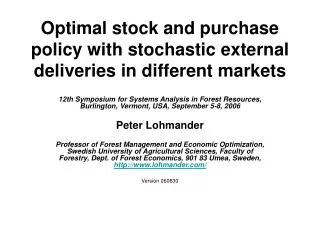
Optimal stock and purchase policy with stochastic external deliveries in different markets. 12th Symposium for Systems Analysis in Forest Resources, Burlington, Vermont, USA, September 5-8, 2006 Peter Lohmander

E N D
Optimal stock and purchase policy with stochastic external deliveries in different markets 12th Symposium for Systems Analysis in Forest Resources, Burlington, Vermont, USA, September 5-8, 2006 Peter Lohmander Professor of Forest Management and Economic Optimization, Swedish University of Agricultural Sciences, Faculty of Forestry, Dept. of Forest Economics, 901 83 Umea, Sweden, http://www.lohmander.com/ Version 060830
Abstract: • Forest industry companies with mills producing pulp, paper and sawn wood often obtain the roundwood from many different sources. These are different with respect to delays and degrees of variation. Private forest owners deliver pulpwood and timber at a stochastic rate. Imported pulpwood and timber may or may not arrive in large quantities a particular day. • The losses may be considerable if mill production has to stop. If the stochastic supply falls, you may instantly reduce the stock level or buy more from the local market. • Large stock level variations are only possible if the average stock is large. Stock holding costs may be considerable. If you control a monopsony and let the amount you buy per period from the local market change over time, this increases the expected cost, since the purchase cost function is strictly convex. In a market with many buyers, the purchase cost function appears almost linear to the individual firm and variations are less expensive. • Hence, the optimal average stock level is higher if we have a monopsony than if we have a market with many independent buyers. • The analysis is based on stochastic dynamic programming in Markov chains via linear programming.
Question:What is the optimal way to control a raw material stock in this typical situation:You have to deliver a constant flow of raw material to a mill. Otherwise, the mill can not run at full capacity utilization, which decreases the revenues very much. Some parts of the deliveries to the raw material stock can not be exactly controlled in the short run. These deliveries are different with respect to delays and degrees of variation.Imported pulpwood and timber may or may not arrive in large quantities a particular day. Some private forest owners deliver pulpwood and timber at a stochastic rate. Some parts of the input to the raw material stock can be rather exactly controlled in the short run. The cost of rapidly changing such input may however be considerable. The costs of such changes are typically a function of the properties of the local raw material market.
The first order optimum condition is: . The second order condition of a unique maximum is satisfied since
The first order optimum condition can be rewritten this way and give us the optimal order quantity as an explicit function of the parameters:
Deterministic multi period linear (and quadratic) programming (LP and QP) models In most cases, such models are based on deterministic assumptions. The degree of detail is high but the solutions can not explicitly take stochastic events into account Adaptive multi period linear (and quadratic) programming models Adaptive optimization is necessary. Compare Lohmander (2002) and Lohmander and Olsson (2004).
The round wood sources and properties Forest industry companies with mills producing pulp, paper and sawn wood often obtain the round wood from many different sources. These are different with respect to delays and degrees of variation.Private forest owners deliver pulpwood and timber at a stochastic rate.Imported pulpwood and timber may or may not arrive in large quantities a particular day. The losses may be considerable if mill production has to stop. If the stochastic supply falls, you may instantly reduce the stock level or buy more from the local market.
Figure The local supply (price) function in the monopsony case.
Now, we will compare two strategies, A and B. In both cases, we have to make sure that the mill can run at full capacity utilization during the following three periods 0, 1 and 2. In strategy A, we try to keep the stock level as low as possible. In strategy B, we buy more wood locally than we instantly need in period 1 in case the entering stock level in period 1 is higher than zero.
The expected present value of strategy A can be illustrated this way, period by period: We can simplify the expression this way:
The expected present value of strategy B can be illustrated this way, period by period:
Let us investigate the difference between the expected present values (costs) of strategies A and B!
Observation 1. • In case the wood market is perfect, no buyer can affect the market price. • This means that it is not economically rational to increase the stock level (strategy B). Strategy A is a better alternative.
Observation 2. In case the wood market is a monopsony, the buyer can affect the market price. This means that Strategy A or strategy B can be the best choice. It is also possible that they are equally good.
If the derivative of price with respect to volume (in the local supply), is sufficiently high in relation to the marginal storage cost, then it is optimal to increase the stock level. Strategy B is better than Strategy A if:
Case 1. Parameters: n = 2 p = ½
The Binomial distribution of exogenous wood deliveries The theory of the Binomial distribution can be found in many textbooks, such as Anderson et al. (2002). The original work on this distribution was made by Jakob Bernoulli (1654-1705).
Case 2. Parameters: n = 6 p = ½
Case 3. Parameters: n = 6 p = ¼
The optimization problem at a general level We want to maximize the expected present value of the profit, all revenues minus costs, over an infinite horizon. This is solved via stochastic dynamic programming. Compare Howard (1960), Wagner (1975), Ross (1983) and Winston (2004).
Min s.t.
The mill In each period, the pulp production volume, prod, is constrained by the capacity of the mill and by the amount of raw material (wood) in the stock. @FOR( s_set(i): @FOR( u_set(j): prod(i,j) = @SMIN( millcap, (s(i)+ u(j))) ));
The cost function contains a setup cost, csetup. The marginal profit in the mill, margprof, is defined as the product price minus variable production costs other than the raw material costs. @FOR( q_set(i): q(i) = i-1); @FOR( q_set(i)|q(i)#LT#1 : Rev(i) = 0); @FOR( q_set(i)|q(i)#GE#1 : Rev(i) = -csetup + margprof*q(i));
The stochastic exogenous deliveries The exogenous deliveries are assumed to have a probability function of the type defined s “Case 2”. The probabilities, pdev, of different deviations, dev, from the expected value are defined in this way: @FOR( b_set(i): dev(i) = i-4 ); @for( b_set(i):@free(dev(i))); pdev(1) = 1/64; pdev(2) = 6/64; pdev(3) = 15/64; pdev(4) = 20/64; pdev(5) = 15/64; pdev(6) = 6/64; pdev(7) = 1/64;
The control function: The company purchase from the local market is the adaptive control, u, in this optimization problem. The instant cost of the control can be calculated via the price function:
The constraints: @FOR( s_set(i): @FOR( u_set(j)| prod(i,j)#LE# millcap #AND# (i+u(j)-prod(i,j))#LE#(smax-10): [w_] w(i) >= Rev(1+prod(i,j)) - c(j) - mcstock*(s(i)+u(j)-prod(i,j)) + d*(pdev(1)*w(i+u(j)-prod(i,j) + 0) + pdev(2)*w(i+u(j)-prod(i,j) + 1) + pdev(3)*w(i+u(j)-prod(i,j) + 2) + pdev(4)*w(i+u(j)-prod(i,j) + 3) + pdev(5)*w(i+u(j)-prod(i,j) + 4) + pdev(6)*w(i+u(j)-prod(i,j) + 5) + pdev(7)*w(i+u(j)-prod(i,j) + 6) ) ));
The parameters: d (=
Optimally controlled stochastic stock path under monopsony or perfect raw material market when the entering stock level state is 0.
Optimally controlled stochastic stock path under monopsony or perfect raw material market when the entering stock level state is 1.
Optimally controlled stochastic stock path under monopsonywhen the entering stock level state is 6.
Optimally controlled stochastic stock path under perfect raw material market when the entering stock level state is 6.
Determination of the steady state probabilities of entering stock states under optimal control and monopsony (with state constraints) • p0 = 1/64*(1*p0 +1*p1 +1*p2 +1*p3); • p1 = 1/64*(6*p0 +6*p1 +6*p2 +6*p3 +1*p4); • p2 = 1/64*(15*p0 +15*p1 +15*p2 +15*p3 +6*p4 +1*p5); • p3 = 1/64*(20*p0 +20*p1 +20*p2 +20*p3 +15*p4 +6*p5 +1*p6 + 1*p7); • p4 = 1/64*(15*p0 +15*p1 +15*p2 +15*p3 +20*p4 +15*p5 +6*p6 +6*p7 + 1*p8); • p5 = 1/64*(6*p0 +6*p1 +6*p2 +6*p3 +15*p4 +20*p5 +15*p6 +15*p7 +6*p8 +1*p9); • p6 = 1/64*(1*p0 +1*p1 +1*p2 +1*p3 +6*p4 +15*p5 +20*p6 +20*p7 +15*p8 +6*p9 +1*p10); • p7 = 1/64*(1*p4 +6*p5 +15*p6 +15*p7 +20*p8 +15*p9 +6*p10); • p8 = 1/64*(1*p5 + 6*p6 + 6*p7 + 15*p8 + 20*p9 +15*p10); • p9 = 1/64*(1*p6 +1*p7 +6*p8 +15*p9 + 20*p10); • p0 + p1 + p2 + p3 + p4 + p5 + p6 + p7 + p8 + p9 + p10 = 1;


![STOCK [EQUITY] MARKETS](https://cdn1.slideserve.com/1829202/stock-equity-markets-dt.jpg)