Chapter 16 Options and Option Strategy
760 likes | 991 Vues
Chapter 16 Options and Option Strategy. By Cheng Few Lee Joseph Finnerty John Lee Alice C Lee Donald Wort. Chapter Outline. 16.1 THE OPTION MARKET AND RELATED DEFINITIONS 16.1.1 What is an Option? 16.1.2 Types of Options and Their Characteristics

Chapter 16 Options and Option Strategy
E N D
Presentation Transcript
Chapter 16Options and Option Strategy By Cheng Few Lee Joseph Finnerty John Lee Alice C Lee Donald Wort
Chapter Outline • 16.1 THE OPTION MARKET AND RELATED DEFINITIONS • 16.1.1 What is an Option? • 16.1.2 Types of Options and Their Characteristics • 16.1.3 Relationships between the Option Price and the Underlying Asset Price • 16.1.4 Additional Definitions and Distinguishing Features • 16.1.5 Types of Underlying Asset • 16.1.6 Institutional Characteristics • 16.2 PUT–CALL PARITY • 16.2.1 European Options • 16.2.2 American Options • 16.2.3 Futures Options • 16.2.4 Market Application
16.3 RISK–RETURN CHARACTERISTICS OF OPTIONS • 16.3.1 Long call • 16.3.2 Short Call • 16.3.3 Long Put • 16.3.4 Short Put • 16.3.5 Long Straddle • 16.3.6 Short Straddle • 16.3.7 Long Vertical (Bull) Spread • 16.3.8 Short Vertical (Bear) Spread • 16.3.9 Calendar (Time) Spreads • 16.4 Excel Approach to Analyze the Option Strategies • 16.4.1 Long Straddle • 16.4.2 Short Straddle • 16.4.3 Long Vertical (Bull) Spread • 16.4.4 Short Vertical (Bear) Spread • 16.4.5 Protective Put • 16.4.6 Covered Call • 16.4.7 Collar • 16.5 Summary 3
16.1 The Option Market and Related Definitions 16.1.1 What is an Option? • An option is a contract conveying the right to buy or sell a designated security at a stipulated price. • The most important element of an option contract is that there is no obligation placed upon the purchaser: it is an “option.” • This attribute of an option contract distinguishes it from other financial contracts.
16.1.2 Types of Options and Their Characteristics • A call option gives its owner the right to buy the underlying asset while a put option conveys to its holder the right to sell the underlying asset. • An option is specified by five essential parts: (1) The type (call or put) (2) The underlying asset (3) The exercise price (4) The expiration date (5) The option price • The exercise price (also called the striking price) is the price stated in the option contract at which the call (put) owner can buy (sell) the underlying asset up to the expiration date, the final calendar date on which the option can be traded.
Table 16.1 Options Quotes for Johnson& Johnson at 03/29/2011
16.1.3 Relationship between the Option Price and the Underlying Asset Price • A call (put) option is said to be in the money if the underlying asset is selling above (below) the exercise price of the option. • An at-the-money call (put) is one whose exercise price is equal to the current price of the underlying asset. • A call (put) option is out of the money if the underlying asset is selling below (above) the exercise price of the option. • The relationship between the price of an option and the price of the underlying asset indicates both the amount of intrinsic value and time value inherent in the option’s price: Intrinsic value = Underlying asset price-Option exercise price • An option’s time value is the amount by which the option’s premium (or market price) exceeds its intrinsic value. • For a call or put option: Time value = Option premium-Intrinsic value where intrinsic value is the maximum of zero or stock price minus exercise price. (16.1) (16.2)
Figure 16.1 The Relationship between an Option’s Exercise Price and its Time Value • In general, the call price should be equal to or exceed the intrinsic value: C Max (S – E, 0) where C = the value of the call option; S = the current stock price; and E = the exercise price.
One more aspect of time value that is very important to discuss is the change in the amount of time value an option has as its duration shortens. • Notice that for the simple care in Figure 16-2 the effect of time decay is smooth up until the last month before expiration, when the time value of an option begins to decay very rapidly. Figure 16.2 The Relationship between Time Value and Time to Maturity for a Near-to-the-Money Option (assuming a Constant Price for the Underlying Asset) 9
Sample Problem 9.1 • It is January 1, the price of the underlying ABC stock is $20 per share, and the time premiums are shown in the following table. • What is the value for the various call options? Call premium = Intrinsic value + Time premium = Max (20-15.0) +50 = $5.50 per share or $550 for 1 contract Table 16.2 Time Premiums Table 16.3 Call Premiums
16.1.4 Additional Definitions and Distinguishing Features • A class of options refers to all call and put options on the same underlying asset. • A series is a subset of a class and consists of all contracts of the same class (such as AT&T) having the same expiration date and exercise price. • When an investor either buys or sells an option (i.e., is long or short) as the initial transaction, the option exchange adds this opening transaction to what is termed the open interest for an option series. • Essentially, open interest represents the number of contracts outstanding at a particular point in time. 11
Volume indicates the number of times a particular option is bought and sold during a particular trading day. • Volume and open interest are measures of an option’s liquidity, the ease with which the option can be bought and sold in large quantities. • Whenever a holder exercises an option, a writer is assigned the obligation to fulfill the terms of the option contract by the exchange on which the option is traded. • If a call holder exercises the right to buy, a call writer is assigned the obligation to sell. • Similarly, when a put holder exercises the right to sell, a put writer is assigned the obligation to buy. 12
16.1.5 Types of Underlying Asset • Although most people would identify common stocks as the underlying asset for an option, a variety of other assets and financial instruments can assume the same function. • The biggest success for options has been realized for options on financial futures. • Options on futures are very similar to options on the actual asset, except that the futures options give their holders the right (not the obligation) to buy or sell predetermined quantities of specified futures contracts at a fixed price within a predetermined period. • While a number of options have existed for various stock-index futures contracts, options now also exist on the stock index itself. • Because of the complexity of having to provide all the stocks in an index at the spot price should a call holder exercise his or her buy right, options on stock indexes are always settled in cash.
16.1.6 Institutional Characteristics • Probably two of the most important underlying factors leading to the success of options have been the standardization of contracts through the establishment of option exchanges and the trading anonymity brought about by the Option Clearing Corporations and clearinghouses of the major futures exchanges. • The sources of futures options traded on the various futures exchanges mentioned earlier are determined by the open-auction bidding, probably the purest form of laissez-faire price determination that can be seen today. • While stock options and options on commodities and indexes are traded in a similar fashion, one major difference prevails — the presence of market makers. • Market makers are individuals who typically trade one type of option for their own account and are responsible for ensuring that a market always exists for their particular contract. • In addition, some option exchanges utilize board brokers as well. • These individuals are charged with the maintenance of the book of limit orders (orders from outside investors that are to be executed at particular prices or when the market goes up or down by a prespecified amount). 14
16.2 Put-Call Parity 16.2.1 European Options • Such relationships among put and call prices are referred to as the put–call parity theorems. • Theorem 1. Put-Call Parity for European Options with No Dividends where: = value of a European call option at time t that matures at time T (T > f); = value of a European put option at time t, that matures at time T; = value of the underlying stock (asset) to both the call and put options at time t; E = exercise price for both the call and put options; = price at time t of a default-free bond that pays $1 with certainty at time T (if it is assumed that this risk-free rate of interest is the same for all maturities and equal to r - in essence a flat-term structure - then = ,under continuous compounding), or = for discrete compounding. (16.3) 15
Equation (16.3) uses the following principle. • If the options are neither dominant nor dominated securities, and if the borrowing and lending rates are equal, then the return patterns of a European call and a portfolio composed of a European put, a pure discount bond with a face value equal to the options exercise price E,and the underlying stock (or asset) are the same. • In understanding why the put–call parity theorem holds, and to support the theorem, two additional properties of option pricing must be provided: • Property 1:At maturity (time T) the call option is worth the greater of ST -E dollars or zero dollars: • Property 2: At maturity, the value of a put option is the greater of E-ST • dollars or zero dollars: (16.4) (16.5) 16
Using the same line of reasoning and argument as for the call option, the second property also implies that the value of a put option is never less than zero. • Table 16.4 provides proof of this first put–call parity theorem. Table 16.4 Call Parity for a European Option with No Dividends
Sample Problem 16.2 • A call option with one year to maturity and exercise price of $110 is selling for $5. • Assuming discrete compounding, a risk-free rate of 10%, and a current stock price of $100, what is the value of a European put option with a strike price of $110 and one-year maturity? Solution
16.2.2 American Options • Theorem 2. Put–Call Parity for an American Option with No Dividends • Sample problem 9.3 A put option with one year to maturity and an exercise price of $90 is selling for $15; the stock price is $100. Assuming discrete compounding and a risk- free rate of 10 percent, what are the boundaries for the price of an American call option? Solution (16.6) 19
16.2.3 Futures Options • Theorem 3.Put–Call Parity for a European Futures Option where is the price at time t for a futures contract maturing at time T (which is the underlying asset to both the call and put options). • Table 16.5 indicates that the argument for this theorem’s proof is similar, with only a few notable exceptions. (16.7) Table 16.5 Put-Call Parity for a European Futures Option 20
16.2.4 Market Application • By combining call options and the underlying security, brokers could construct a synthetic put. • To illustrate, the put–call parity theorem is used when a futures contract is the underlying asset. • Furthermore, to simulate the option broker’s circumstances on July 1, 1984, the equation is merely rearranged to yield the put’s “synthetic” value: • So instead of a futures contract being purchased, it is sold. • Assume the following values and use the S&P 500 index futures as the underlying asset. E = 155.00 (16.8) 21
16.3 Risk-Return Characteristics of Options 16.3.1 Long Call • Figure 16.3 illustrates the profit profile of a long call position. • The following summarizes the basic risk–return features for a long-call position. • Profit potential: unlimited. • Loss potential: limited (to cost of option). • Effect of time decay: negative (decrease option’s value). • Market expectation: bullish. 22
Figure 16.3 Profit Profile for a Long Call • As the profit profile indicates, the time value of a long call declines over time.
16.3.2 Short Call • Selling a call (writing it) has risk–reward characteristics, which are the inverse of the long call. • However, one major distinction arises when writing calls (or puts) rather than buying them. • That is, the writer can either own the underlying asset upon which he or she is selling the option (a covered write), or simply sell the option without owning the asset (a naked write). • Let us first examine the profit profile and related attributes of the naked short call, displayed in Figure 16.4. • The following summarizes the basic risk–return features for a naked short-call position. • Profit potential: limited (to option premium). • Loss potential: unlimited. • Effect of time decay: positive (makes buyer’s position less valuable). • Market expectation: bearish to neutral. 24
Now consider the other type of short-call position, covered-call writing. • Because the seller of the call owns the underlying asset in this case, the risk is truncated. • The purpose of writing a call on the underlying asset when it is owned is twofold. • The profit profile for a covered short call (or a covered write) in Figure 16.5 provides further illustration. • The following summarizes the basic risk–return features for the covered short-call position. • Profit potential: limited (exercise price − asset price + call premium). • Loss potential: limited (asset price − call premium). • Effect of time decay: positive. • Market expectation: neutral to mildly bullish. 26
16.3.3 Long Put • Again, the put option conveys to its purchasers the right to sell a given quantity of some asset at a prespecified price on or before its expiration date. • Similar to a long call, a longput is also a highly leveraged position, but the purchaser of the put makes money on the investment only when the price of the underlying asset declines. • The profit profile for a long put is seen in Figure 16.6. • The following summarizes the basic risk–return features for the profit profile of a long-put position. • Profit potential: limited (asset price must be greater than zero). • Loss potential: limited (to cost of put). • Effect of time decay: negative or positive. • Market expectation: bearish. 28
16.3.4 short Put • As was true for the short-call position, put writing can be covered or uncovered (naked). • The risk–return features of the uncovered (naked) short put are discussed first. • For taking on the obligation to buy the underlying asset at the exercise price, the put writer receives a premium. • The maximum profit for the uncovered-put-writer is this premium, which is initially received. • Figure 16.7 provides further illustration. • The following summarizes the basic risk–return features for the profit profile of an uncovered short-put position. • Profit potential: limited (to put premium). • Loss potential: limited (asset price must be greater than zero). • Effect of time decay: positive or negative. • Market expectation: neutral to bullish. 30
16.3.5 Long Straddle • A straddle is a simultaneous position in both a call and a put on the same underlying asset. • A long straddle involves purchasing both the call and the put. • By combining these two seemingly opposing options, an investor can get the best risk–return combination that each offers. • The profit profile for a long straddle in Figure 16.8 illustrates the nature of this synthetic asset. • The following summarizes the basic risk–return features for the profit profile of a long-straddle position. • Profit potential: unlimited on upside, limited on downside. • Loss potential: limited (to cost of call and put premiums). • Effect of time decay: negative. • Market sentiment: bullish or bearish. 32
Sample problem 16.4 Situation: • An investor feels the stock market is going to break sharply up or down but is not sure which way. • However, the investor is confident that market volatility will increase in the near future. • To express his position, the investor puts on a long straddle using options on the S&P 500 index, buying both at-the-money call and put options on the September contract. • The current September S&P 500 futures contract price is 155.00. • Assume the position is held to expiration.
Transaction: 1. Buy 1 September 155 call at $2.00. ($1,000) 2. Buy 1 September 155 put at $2.00. ($1,000) Net initial investment (position value) ($2,000) Results: 1. If futures price = 150.00: (a) 1 September call expires at $0. ($1,000) (b) 1 September put expires at $5.00. $2,500 (c) Less initial cost of put ($1,000) Ending position value (net profit) $ 500
Results: 2. If futures price = 155.00: (a) 1 September call expires at $0. ($1,000) (b) 1 September put expires at $0. ($1,000) Ending position value (net loss) ($2,000) 3. If futures price = 160.00: (a) 1 September call expires at $5.00 $2,500 (b) 1 September call expires at $0. ($1,000) (c) Less initial cost of put ($1,000) Ending position value (net profit) $ 500
Summary: Maximum profit potential: unlimited. If the market had contributed to move below 150.00 or above 160.00, the position would have continued to increase in value. Maximum loss potential: $2,000, the initial investment. Breakeven points: 151.00 and 159.00, for the September S&P 500 futures contract. Effect of time decay: negative, as evidenced by the loss incurred, with no change in futures price (result 2)
16.3.6 Short Straddle • A short straddle is a simultaneous position in both a short call and a short put on the same underlying asset. • Contrary to the long-straddle position, selling a straddle can be an effective strategy when an investor expects little or no movement in the price of the underlying asset. • Figure 16.9 shows the short straddle’s profit profile. • The following summarizes the basic risk–return features for the profit profile of a short-straddle position. • Profit potential: limited (to call and put premiums). • Loss potential: unlimited on upside, limited on downside. • Effect of time decay: positive. • Market expectation: neutral. 38
Sample problem 16.5 Situation: • An investor feels the market is overestimating price volatility at the moment and that prices are going to remain stable for some time. • To express his opinion, the investor sells a straddle consisting of at-the-money call and put options on the September S&P 500 futures contract, for which the current price is 155.00. • Assume the position is held to expiration. Transaction: 1. Sell 1 September 155 call at $2.00 (x $500 per point). $1,000 2. Sell 1 September 155 put at $2.00. $1,000 Net initial inflow (position value) $2,000
Results: 1. If futures price = $150.00: (a) 1 September 155 call expires at 0. $1,000 (b) I September 155 put expires at $5.00. ($2,500) (c) Plus initial inflow from sale of put $1,000 Ending position value (net loss) ($ 500) 2. If futures price = $155.00: (a) 1 September 155 call expires at 0. $1,000 (b) I September 155 put expires at 0. $1,000 Ending position value (net profit) $2,000
Results: 3. If futures price = 160.00: (a) 1 September 155 call expires at $5.00. ($2,500) (b) I September put expires at 0. $1,000 (c) Plus initial inflow from sale of call $1,000 Ending position value (net loss) ($ 500) Summary: Maximum profit potential: $2,000, result 2. where futures price does not move. Maximum loss potential: unlimited. If futures price had continued up over 160.00 or down below 145.00, this position would have kept losing money. Breakeven points: 151.00 and 159.00, an eight-point range for profitability of the position. Effect of time decay: positive, as evidenced by result 2. 42
16.3.7 Long Vertical (Bull) Spread • When dealing strictly in options, a spread is a combination of any two or more of the same type of options (two calls or two puts, for instance) on the same underlying asset. • A long vertical spread is also known as a bull spread because of the bullish market expectation of the investor who enters into it. • An examination of the profit profile for the long vertical spread (see Figure 16.10) can tell more about its risk–return attributes. • The following summarizes the basic risk–return features for the profit profile of a long-vertical-spread position. • Profit potential: limited (up to the higher exercise price). • Loss potential: limited (down to the lower exercise price) • Effect of time decay: mixed. • Market expectation: cautiously bullish. 43
Sample problem 9.6 Situation: • An investor is moderately bullish on the West German mark. • He would like to be long but wants to reduce the cost and risk of this position in case he is wrong. • To express his opinion, the investor puts on a long vertical spread by buying a lower-exercise-price call and selling a higher-exercise-price call with the same month to expiration. • Assume the position is held to expiration. Transaction: 1. Buy 1 September 0.37 call at 0.0047 (x 125.000 per point). ($ 587.50) 2. Sell 1 September 0.38 call at 0.0013. $ 162.50 Net initial investment (position value) ($ 425.00)
Results: 1. If futures price = 0.3700: (a) 1 September 0.37 call expires at 0. ($ 587.50) (b) 1 September 0.38 call expires at 0. $ 162.50 Ending position value (net loss) ($ 425.00) 2.If futures price = 0.3800: (a) 1 September 0.37 call expires at 0.0100. $1,250.00 (b) I September 0.38 call expires at 0. $ 162.50 Less initial cost of 0.37 call ($ 587.50) Ending position value (net profit) $ 825.00 3. If futures price = 0.3900: (a) 1 September 0.38 call expires at 0.0200. $2,500.00 (b) 1 September put expires at 0. ($1,250.00) Less initial premium of 0.37 call ($ 587.50) Plus initial premium of 0.38 call $ 162.50 Ending position value (net profit) ($ 825.00)
Summary: Maximum profit potential: $825.00, result 2. Maximum loss potential: $425.00, result 1. Breakeven point: 0.3734. Effect of time decay: mixed. positive if price is at high end of range and negative if at low end.
16.3.8 Short Vertical (Bear) Spread • The short vertical spread is simply the reverse of the corresponding long position. • That is, an investor buys a high-exercise-price call (or put) and sells a low-exercise-price call (or put), both having the same time to expiration left. • As the more common name for this type of option position is bear spread, it is easy to infer the type of market sentiment consistent with this position. • The profit profile for the short vertical spread is seen in Figure 16.11. • The following summarizes the basic risk–return features for the profit profile of a short-vertical-spread position. • Profit potential: limited (down to ). • Loss potential: limited (up to ). • Effect of time decay: mixed (opposite to that of long vertical spread). • Market sentiment: mildly bearish. 48
16.3.9 Calendar (Time) Spreads • A calendar spread (also called a time or horizontal spread) consists of the sale of one option and the simultaneous purchase of another option with the same exercise price but a longer term to maturity. • The objective of the calendar spread is to capture the faster erosion in the time-premium portion of the shorted nearer-term-to-maturity option. • Figure 16.12 displays the calendar spread’s profit profile and related risk–return attributes. • The following summarizes the basic risk–return features for the profit profile of a neutral calendar- spread position. • Profit potential: limited. • Loss potential: limited (to original cost of position). • Effect of time decay: positive. (Option sold loses value faster than option bought.) • Market sentiment: neutral. 50