Lecture 4: Dynamic routing protocols
Lecture 4: Dynamic routing protocols. Today: Overview of router architecture RIP, OSPF, BGP Notes on Lab 4 Midterm review. Router Architectures. An overview of router architectures. Two key router functions. Control plane: run routing protocols (RIP, OSPF, BGP).

Lecture 4: Dynamic routing protocols
E N D
Presentation Transcript
Lecture 4: Dynamic routing protocols Today: Overview of router architecture RIP, OSPF, BGP Notes on Lab 4 Midterm review
Router Architectures An overview of router architectures.
Two key router functions Control plane: run routing protocols (RIP, OSPF, BGP) Data plane:forwarding packets from incoming to outgoing link
Routing and Forwarding Routing functions include: • route calculation • maintenance of the routing table • execution of routing protocols • On commercial routers handled by a single general purpose processor, called route processor IP forwarding is per-packet processing • On high-end commercial routers, IP forwarding is distributed • Most work is done on the interface cards
Hardware components of a router: Network interfaces Switching fabrics Processor with a memory and CPU Processor Memory CPU Switching fabric Interface Card Interface Card Interface Card Router Hardware Components
On a PC router: Switching fabric is the (PCI) bus Interface cards are NICs (e.g., Ethernet cards) All forwarding and routing is done on central processor On Commercial routers: Switching fabrics and interface cards can be sophisticated Central processor is the route processor (only responsible for control functions) Processor Memory CPU Switching fabric Interface Card Interface Card Interface Card PC Router versus commercial router
Evolution of Router Architectures • Early routers were essentially general purpose computers • Today, high-performance routers resemble supercomputers • Exploit parallelism • Special hardware components • Until 1980s (1st generation): standard computer • Early 1990s (2nd generation): delegate to interfaces • Late 1990s (3rd generation): Distributed architecture • Today: Distributed over multiple racks
1st Generation Routers (switching via memory) • This architecture is still used in low end routers • Arriving packets are copied to main memory via direct memory access (DMA) • Switching fabric is a backplane (shared bus) • All IP forwarding functions are performed in the central processor. • Routing cache at processor can accelerate the routing table lookup.
Memory Input Port Output Port System Bus Drawbacks of 1st Generation Routers • Forwarding Performance is limited by memory and CPU • Capacity of shared bus limits the number of interface cards that can be connected
2nd Generation Routers (switching via a shared bus) • Keeps shared bus architecture, but offloads most IP forwarding to interface cards • Interface cards have local route cache and processing elements Fast path:If routing entry is found in local cache, forward packet directly to outgoing interface Slow path:If routing table entry is not in cache, packet must be handled by central CPU
Another 2nd Generation Architecture • IP forwarding is done by separate components (Forwarding Engines) Forwarding operations: • Packet received on interface: Store the packet in local memory. Extracts IP header and sent to one forwarding engine • Forwarding engine does lookup, updates IP header, and sends it back to incoming interface • Packet is reconstructed and sent to outgoing interface.
Drawbacks of 2nd Generation Routers Bus contention limits throughput
3rd Generation Architecture • Switching fabric is an interconnection network (e.g., a crossbar switch) • Distributed architecture: • Interface cards operate independent of each other • No centralized processing for IP forwarding • These routers can be scaled to many hundred interface cards and to aggregate capacity of > 1 Terabit per second
Slotted Chassis • Large routers are built as a slotted chassis • Interface cards are inserted in the slots • Route processor is also inserted as a slot • This simplifies repairs and upgrades of components
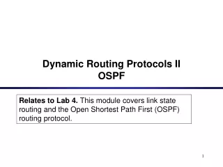
Dynamic Routing ProtocolsPart 1: RIP Relates to Lab 4. The first module on dynamic routing protocols. This module introduces RIP.
Routing • Recall: There are two parts to routing IP packets: 1. How to pass a packet from an input interface to the output interface of a router (packet forwarding) ? 2. How to find and setup a route ? • We already discussed the packet forwarding part • Longest prefix match • There are two approaches for calculating the routing tables: • Static Routing (Lab 3) • Dynamic Routing: Routes are calculated by a routing protocol
Routing protocols versus routing algorithms • Routing protocols establish routing tables at routers. • A routing protocol specifies • What messages are sent between routers • Under what conditions the messages are sent • How messages are processed to compute routing tables • At the heart of any routing protocol is a routing algorithm that determines the path from a source to a destination
What routing algorithms common routing protocols use Routing algorithm Routing protocol
Intra-domain routing versus inter-domain routing • Recall Internet is a network of networks. • Administrative autonomy • internet = network of networks • each network admin may want to control routing in its own network • Scale: with 200 million destinations: • can’t store all dest’s in routing tables! • routing table exchange would swamp links
Autonomous systems • aggregate routers into regions, “autonomous systems” (AS) or domain • routers in the same AS run the same routing protocol • “intra-AS” or intra-domain routing protocol • routers in different AS can run different intra-AS routing protocol
Autonomous Systems • An autonomous system is a region of the Internet that is administered by a single entity. • Examples of autonomous regions are: • UCI’s campus network • MCI’s backbone network • Regional Internet Service Provider • Routing is done differently within an autonomous system (intradomain routing) and between autonomous system (interdomain routing). • RIP, OSPF, IGRP, and IS-IS are intra-domain routing protocols. • BGP is the only inter-domain routing protocol.
RIP and OSPF computes shortest paths • Shortest path routing algorithms • Goal: Given a network where each link is assigned a cost. Find the path with the least cost between two nodes. b 1 3 2 a c d 6
Distance vector algorithm • A decentralized algorithm • A router knows physically-connected neighbors and link costs to neighbors • A router does not have a global view of the network • Path computation is iterative and mutually dependent. • A router sends its known distances to each destination (distance vector) to its neighbors. • A router updates the distance to a destination from all its neighbors’ distance vectors • A router sends its updated distance vector to its neighbors. • The process repeats until all routers’ distance vectors do not change (this condition is called convergence).
A router updates its distance vectors using bellman-ford equation Bellman-Ford Equation Define dx(y) := cost of the least-cost path from x to y Then • dx(y) = minv{c(x,v) + dv(y) }, where min is taken over all neighbors of node x
Distance vector algorithm: initialization • Let Dx(y) be the estimate of least cost from x to y • Initialization: • Each node x knows the cost to each neighbor: c(x,v). For each neighbor v of x, Dx(v) = c(x,v) • Dx(y) to other nodes are initialized as infinity. • Each node x maintains a distance vector (DV): • Dx = [Dx(y): y 2 N ]
Distance vector algorithm: updates • Each node x sends its distance vector to its neighbors, either periodically, or triggered by a change in its DV. • When a node x receives a new DV estimate from a neighbor v, it updates its own DV using B-F equation: • If c(x,v) + Dv(y) < Dx(y) then • Dx(y) = c(x,v) + Dv(y) • Sets the next hop to reach the destination y to the neighbor v • Notify neighbors of the change • The estimate Dx(y) will converge to the actual least cost dx(y)
Distance vector algorithm: an example • t = 0 • a = ((a, 0), (b, 3), (c, 6)) • b = ((a, 3), (b, 0), (c,1)) • c = ((a, 6), (b, 1), (c, 0) (d, 2)) • d = ((c, 2), (d, 0)) b 1 3 2 a c d 6 • t = 1 • a = ((a, 0), (b, 3), (c, 4), (d, 8)) • b = ((a, 3), (b, 0), (c,1), (d, 3)) • c = ((a, 4), (b, 1), (c, 0), (d, 2)) • d = ((a, 8), (b, 3), (c, 2), (d,0)) • t = 2 • a = ((a, 0), (b, 3), (c, 4), (d, 6)) • b = ((a, 3), (b, 0), (c,1), (d, 3)) • c = ((a, 4), (b, 1), (c, 0), (d, 2)) • d = ((a, 6), (b, 3), (c, 2), (d,0))
How to map the abstract graph to the physical network • Nodes (e.g., v, w, n) are routers, identified by IP addresses, e.g. 10.0.0.1 • Nodes are connected by either a directed link or a broadcast link (Ethernet) • Destinations are IP networks, represented by the network prefixes, e.g., 10.0.0.0/16 • Net(v,n) is the network directly connected to router v and n. • Costs (e.g. c(v,n)) are associated with network interfaces. • Router1(config)# router rip • Router1(config-router)# offset-list 0 out 10 Ethernet0/0 • Router1(config-router)# offset-list 0 out 10 Ethernet0/1
Distance vector routing protocol: Routing Table c(v,w): cost to transmit on the interface to network Net(v,w) Net(v,w): Network address of the network between v and w D(v,net) is v’s cost to Net
Distance vector routing protocol: Messages [Net , D(v,Net)] v n • Nodes send messages to their neighbors which contain distance vectors • A message has the format: [Net , D(v,Net)] means“My cost to go to Net is D (v,Net)”
Distance vector routing algorithm: Sending Updates Periodically, each node v sends the content of its routing table to its neighbors:
Initiating Routing Table I • Suppose a new node v becomes active. • The cost to access directly connected networks is zero: • D (v, Net(v,m)) = 0 • D (v, Net(v,w)) = 0 • D (v, Net(v,n)) = 0
Initiating Routing Table II • Node v sends the routing table entry to all its neighbors:
Initiating Routing Table III • Node v receives the routing tables from other nodes and builds up its routing table
Updating Routing Tables I • Suppose node v receives a message from node m:[Net,D(m,Net)] Node v updates its routing table and sends out further messagesif the message reduces the cost of a route: • if ( D(m,Net) + c (v,m) < D (v,Net) ) { Dnew (v,Net) := D(m,Net) + c (v,m);Update routing table; send message [Net, Dnew (v,Net)] to all neighbors }
Updating Routing Tables II • Before receiving the message: • Suppose D(m,Net) + c (v,m) < D (v,Net):
Assume: - link cost is 1, i.e., c(v,w) = 1 - all updates, updates occur simultaneously - Initially, each router only knows the cost of connected interfaces Example 10.0.1.0/24 10.0.2.0/24 10.0.3.0/24 10.0.4.0/24 10.0.5.0/24 .2 .1 .2 .1 .2 .1 .2 .1 Router A Router B Router C Router D cost cost cost cost Net via Net via Net via Net via t=0:10.0.1.0 - 010.0.2.0 - 0 t=0:10.0.2.0 - 010.0.3.0 - 0 t=0:10.0.3.0 - 010.0.4.0 - 0 t=0:10.0.4.0 - 010.0.5.0 - 0 t=1:10.0.1.0 - 010.0.2.0 - 0 10.0.3.0 10.0.2.2 1 t=1:10.0.1.0 10.0.2.1 1 10.0.2.0 - 010.0.3.0 - 010.0.4.0 10.0.3.2 1 t=1:10.0.2.0 10.0.3.1 1 10.0.3.0 - 010.0.4.0 - 010.0.5.0 10.0.4.2 1 t=1:10.0.3.0 10.0.4.1 110.0.4.0 - 010.0.5.0 - 0 t=2:10.0.1.0 - 010.0.2.0 - 0 10.0.3.0 10.0.2.2 110.0.4.0 10.0.2.2 2 t=2:10.0.1.0 10.0.2.1 1 10.0.2.0 - 010.0.3.0 - 010.0.4.0 10.0.3.2 110.0.5.0 10.0.3.2 2 t=2:10.0.1.0 10.0.3.1 2 10.0.2.0 10.0.3.1 1 10.0.3.0 - 010.0.4.0 - 010.0.5.0 10.0.4.2 1 t=2:10.0.2.0 10.0.4.1 210.0.3.0 10.0.4.1 110.0.4.0 - 010.0.5.0 - 0
Example 10.0.1.0/24 10.0.2.0/24 10.0.3.0/24 10.0.4.0/24 10.0.5.0/24 .2 .1 .2 .1 .2 .1 .2 .1 Router A Router B Router C Router D cost cost cost cost Net via Net via Net via Net via t=2:10.0.2.0 10.0.4.1 210.0.3.0 10.0.4.1 110.0.4.0 - 010.0.5.0 -0 t=2:10.0.1.0 - 010.0.2.0 - 0 10.0.3.0 10.0.2.2 110.0.4.0 10.0.2.2 2 t=2:10.0.1.0 10.0.2.1 1 10.0.2.0 - 010.0.3.0 - 010.0.4.0 10.0.3.2 110.0.5.0 10.0.3.2 2 t=2:10.0.1.0 10.0.3.1 2 10.0.2.0 10.0.3.1 1 10.0.3.0 - 010.0.4.0 - 010.0.5.0 10.0.4.2 1 t=3:10.0.1.0 10.0.2.1 1 10.0.2.0 - 010.0.3.0 - 010.0.4.0 10.0.3.2 110.0.5.0 10.0.3.2 2 t=3:10.0.1.0 - 010.0.2.0 - 0 10.0.3.0 10.0.2.2 110.0.4.0 10.0.2.2 210.0.5.0 10.0.2.2 3 t=3:10.0.1.0 10.0.4.1 310.0.2.0 10.0.4.1 210.0.3.0 10.0.4.1 110.0.4.0 - 010.0.5.0 - 0 t=3:10.0.1.0 10.0.3.1 2 10.0.2.0 10.0.3.1 1 10.0.3.0 - 010.0.4.0 - 010.0.5.0 10.0.4.2 1 Now, routing tables have converged !
Characteristics of Distance Vector Routing Protocols • Periodic Updates: Updates to the routing tables are sent at the end of a certain time period. A typical value is 30 seconds. • Triggered Updates: If a metric changes on a link, a router immediately sends out an update without waiting for the end of the update period. • Full Routing Table Update: Most distance vector routing protocol send their neighbors the entire routing table (not only entries which change). • Route invalidation timers: Routing table entries are invalid if they are not refreshed. A typical value is to invalidate an entry if no update is received after 3-6 update periods.
The Count-to-Infinity Problem A 1 B 1 C A's Routing Table B's Routing Table via via to cost to cost (next hop) (next hop) C B 2 C C 1 now link B-C goes down 1 C B 2 C - 1 C 2 C 1 C - C A 3 1 C C 3 1 C B 4 C - 1 C 4 C
Count-to-Infinity • The reason for the count-to-infinity problem is that each node only has a “next-hop-view” • For example, in the first step, A did not realize that its route (with cost 2) to C went through node B • How can the Count-to-Infinity problem be solved?
Count-to-Infinity • The reason for the count-to-infinity problem is that each node only has a “next-hop-view” • For example, in the first step, A did not realize that its route (with cost 2) to C went through node B • How can the Count-to-Infinity problem be solved? • Solution 1: Always advertise the entire path in an update message to avoid loops (Path vectors) • BGP uses this solution
Count-to-Infinity • The reason for the count-to-infinity problem is that each node only has a “next-hop-view” • For example, in the first step, A did not realize that its route (with cost 2) to C went through node B • How can the Count-to-Infinity problem be solved? • Solution 2:Never advertise the cost to a neighbor if this neighbor is the next hop on the current path (Split Horizon) • Example: A would not send the first routing update to B, since B is the next hop on A’s current route to C • Split Horizon does not solve count-to-infinity in all cases! • You can produce the count-to-infinity problem in Lab 4.
RIP - Routing Information Protocol • A simple intradomain protocol • Straightforward implementation of Distance Vector Routing • Each router advertises its distance vector every 30 seconds (or whenever its routing table changes) to all of its neighbors • RIP always uses 1 as link metric • Maximum hop count is 15, with “16” equal to “” • Routes are timeout (set to 16) after 3 minutes if they are not updated
RIP - History • Late 1960s : Distance Vector protocols were used in the ARPANET • Mid-1970s: XNS (Xerox Network system) routing protocol is the ancestor of RIP in IP (and Novell’s IPX RIP and Apple’s routing protocol) • 1982 Release of routed for BSD Unix • 1988 RIPv1 (RFC 1058) - classful routing • 1993 RIPv2 (RFC 1388) - adds subnet masks with each route entry - allows classless routing • 1998 Current version of RIPv2 (RFC 2453)
RIPv1 Packet Format 1: RIPv1 1: request2: response 2: for IP Address of destination Cost (measured in hops) One RIP message can have up to 25 route entries
RIPv2 • RIPv2 is an extends RIPv1: • Subnet masks are carried in the route information • Authentication of routing messages • Route information carries next-hop address • Uses IP multicasting • Extensions of RIPv2 are carried in unused fields of RIPv1 messages
RIPv2 Packet Format 2: RIPv2 1: request2: response 2: for IP Address of destination Cost (measured in hops) One RIP message can have up to 25 route entries
RIPv2 Packet Format 2: RIPv2 Used to provide a method of separating "internal" RIP routes (routes for networks within the RIP routing domain) from "external" RIP routes Subnet mask for IP address Identifies a better next-hop address on the same subnet than the advertising router, if one exists (otherwise 0….0)