Download

1 / 45
450 likes | 614 Vues
Techniques for Organization and Visualization of Community Photo Collections. Kumar Srijan Faculty Advisor : Dr. C.V . Jawahar. Community Photo Collections. Anyone can take photographs! Sharing photographs is easy! Searching for photographs is easy!. Community Photo Collections.

E N D
Techniques for Organization and Visualization of Community Photo Collections Kumar Srijan Faculty Advisor : Dr. C.V. Jawahar
Community Photo Collections • Anyone can take photographs! • Sharing photographs is easy! • Searching for photographs is easy!
Community Photo Collections • Golkonda Fort (Google Images + Flickr) • > 50 K images
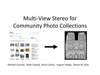
Photo Tourism • Noah Snavely, Steven M. Seitz, Richard Szeliski • Photo tourism: Exploring photo collections in 3D • Photosynth
Photo Tourism Input Images Computing Correspondences Pairwise Feature Matching Match Refinement Feature Extraction Track Creation Incremental SfM Seeding Add new images and triangulate new points Bundle adjust Full Scene Reconstruction Snavely et. al, Photo Tourism: Exploring image collections in 3D
Bottlenecks and Issues • Quadratic Image Matching cost • Global scene reconstruction • O(N4) in the worst case • Sensitivity to the choice of the initial pair • Cascading of errors Image credits: Snavely et. al, Photo Tourism: Exploring image collections in 3D
Bottlenecks and Issues • Timing Breakdown Full Scene Reconstruction for Trafalgar Square with 8000 images took > 50 days Snavely et. al, Photo Tourism: Exploring image collections in 3D
Motivation • CPCs are unstructured collections • Different resolutions, viewpoint , lighting conditions… • Very limited number of images match • Contribution 1 : Matching • Exhaustive pairwise matching w/oquadratic cost • Contribution 2 : Visualization • Framework for bypassing the issues faced with Incremental Sfm.
Image Matching Problem • Compute Image Match Graph • Images Nodes • Image Match Edges • Queries: • Connected components • Shortest path
Discovering Matching Images • Object Retrieval with Large Vocabularies and Fast Spatial Matching – Philbin et al. • Image Retrieval 1. Indexing Image Database • Quantization : Image Features Visual Words(VW) • Inverted Index : over VWs 2. Querying Image Database • Filtering Shortlist of Top Scoring matches • Verification of shortlist • O(N) time for a single querying
Discovering Matching Images • Large Scale Discovery of Spatially Related Images - Chum, O. and Matas. J
Our Solution : Overview • Exhaustive Pairwise Matching • Query each image in turn • Goal : O(1) per query • Addressing Exhaustiveness • Verify all potential matches : No shortlists • Verification doable from Index retrievals • Our Main Result :Indexing geometry allows both!
Indexing Geometry • High Order Features • Combine nearby features • PrimarywithSecondary Features • Encode Affine Invariants • Relative Orientation and Scale • Normalized distance • Baseline orientation • HOF is a Tuple • <VWp,VWs,g1,g2,g3,g4> • Huge Feature Space
Constant Time Queries using HOFs • Regular Inverted Index • Posting lists grow with Database size O(N) • HOF => Huge Feature Space ( > 1012 ) • Reproject with Hash Functions! • Range α Database size • Constant sized posting lists • Result :Constant time queries
Spatial Verification • Computable from index retrievals • For a query primary feature • Search all secondary features in database images • Pass if R features are found.
Solution : Summary • Extract HoF in the N database images • Select Reprojectionsize as CN • Initialize an Index of size CN • Indexing • Key : Hash value ofHoF • Value : Image Id • Query : Each image in turn • Record matches in adjacency list • Result : Image Match Graph
Results • UK benchmark • 2550 categories x 4 = 10400 images • 73.2 % recall • Large Scale Discovery of Spatially Related Images (Min Hash based solution) • 49.6 % recall
Results • Small Clusters • Errors
Problem Statement • Efficiently browse and keep Incorporating incoming stream of images
Our Solution : Overview Independent Partial Scene Reconstructions instead of Global Scene Reconstruction • Observation : In a walkthrough, users primarily see nearby overlapping images. • Advantages: • Robustness to errors in incremental SfM module • Worst case linear running time • Scalable • Incremental
Partial Reconstructions Compute partial Reconstructions Compute Matches Refine Matches Incorrect Match Correct Match Image Match Standard SfM
User interface and navigation Sample image Input images Verified neighbors Partial reconstruction Visualization Interface
Incremental insertion Geometric Verification Match Compute Partial Scene Reconstruction New Image Improve Connectivity
Dataset Golconda Fort, Hyderabad Fort Dataset 5989 images
Results • Courtyard Dataset with 687 images • Initialized with 200 images • Added 487 image one by one • Largest CC of 674 images.
Conclusions • Image Matching : HOFs gives a larger feature space which can be reprojected to obtain sparse posting lists making Exhaustive Pairwise Matching feasible. • CPCs Visualization : Partial scene reconstructions can effectively be used to navigate through large collections of images. • Bypasses issues faced by standard Sfm.
Thank you! • QUESTIONS ?! • Take Home Message : 2 ideas • For information retrieval using a inverted index, combining features gives a larger feature space which can be reprojected to control the average lengths of posting lists, and thus the query time. • For a very complex algorithm O(N > 2), it may sometimes be meaningful to fragment the dataset into O(N) groups, each of finite size, there by reducing the overall complexity to O(N).
Thank You! • Questions
Photo Tourism • Annotation Transfer
Matching images • Correspondence computation • Match Verification • RANSAC based epipolar geometry estimation • Expensive
Establishing Correspondences • SIFT features : D. Lowe • Scale Invariant Feature Transform • Key points • Detection • Description : 128D • Correspondence • Key points with Similar descriptors • Alternatives : SURF, Brisk..
Image Retrieval • Feature Quantization • Visual Words A B C D E F G B C F A D E G
Image Retrieval • Feature Quantization • Visual Words • Inverted Indexing Query visual Word (E)
Image Retrieval • Feature Quantization • Visual Words • Inverted Indexing • Geometric verification • Epipolar Geometry
Bloom Filters • Bloom Filter • Set Membership • Bit array(m) • Hash Functions(k) • Elements(n) • Insert(A) 0 0 0 0 H1 0 A H2 0 H3 0 0 0 0 0 0
Bloom Filters • Bloom Filter • Set Membership • Bit array(m) • Hash Functions(k) • Elements(n) • Insert(A) 0 1 0 0 H1 0 A H2 0 H3 0 0 1 1 0 0
Bloom Filters • Bloom Filter • Set Membership • Bit array(m) • Hash Functions(k) • Elements(n) • Insert(A) • Insert(B) 0 1 0 0 H1 1 B H2 0 H3 0 0 1 1 1 0
Bloom Filters • Bloom Filter • Set Membership • Bit array(m) • Hash Functions(k) • Elements(n) • Insert(A) • Insert(B) • Query(C) • Not present Set = {A,B} 0 1 0 0 H1 1 C H2 0 H3 0 0 1 1 1 0
Bloom Filters • Bloom Filter • Set Membership • Bit array(m) • Hash Functions(k) • Elements(n) • Insert(A) • Insert(B) • Query(C) • Not present • Query(D) • False positive Set = {A,B} 0 1 0 0 H1 1 D H2 0 H3 0 0 1 1 1 0
Global vs. Partial • Global : Allows transition to any image • Partial : Allows transition to a limited number of overlapping images • A -> B implies B -> A A A B B