Download
1 / 19
190 likes | 268 Vues
This study analyzes the geometric features of Eruptive Flux-Rope (EFR) models in coronagraph CME images, determining flux-rope orientations, density profiles, and magnetic field characteristics. The research proposes an elliptical flux-rope model fit using Krall and St. Cyr's geometric approach, and discusses the relationship between magnetic fields in active regions and magnetic clouds. The modified EFR model presents insights into the density, physics, and geometry of the flux ropes, offering a comprehensive understanding of their structure.

E N D
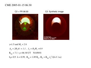
CME 2005-01-15 06:30 C2 + FR 06:30 C2: Synthetic image =1.5 and Ms = 2.8 = 2R1/d = 1.1 , = R2/R1 =0.9 Rtip = 7.1 t1= 06:30 UT N16W01 b0= 0.9 = 0.59, Rsh = 1.89 R0 , R0= Rtip/(2+1/ )
CME 2005-01-15 06:30 C3 + FR 07:42 C3: Synthetic image =1.5 and Ms = 3.5 = 2R1/d = 1.1 = R2/R1 =0.9 Rtip = 25.3 t1= 07:42 UT N20W00 b0= 0.7 = 1.76, Rsh = 1.74 R0 , R0 = Rtip/(2+1/ )
Eruptive Flux-Rope (EFR)(Chen 1996) The magnetic field is given by: Bp(r) = 3Bp(r/a)(1-(r/a)^2+r^4/(3a^4) Geometry showing that a FR consists of the current core a and the Bp while Bex outlines the boundary of the FR [Chen et al. , 1996].
Eruptive Flux-Rope (EFR)(Chen 1996, Krall et al., 2006) The magnetic field of EFR is given by: Geometry showing that a FR consists of the current core a and the Bp while Bex outlines the boundary of the FR [Chen et al. , 1996]. Where Bp = Bp(a) is the poloidal field and Bt is the average of toroidal field Bt(r) across the minor radius, with the Relation Bt(0) = 3Bt. The toroidal current-carrying (a ) loop model yields Bp, Bt, and a, which are used to specify the solution.
Relation to coronagraph CME images: 1) Core: a central current-channel (r = a) and prominence. 2) Cavity : a density depletion around a central current-channel (r = a) that produces the magnetic-cloud-like fields at 1 AU. 3) Rim: Overlapped external loops and shock wave disturbance . (a) (b) (c) (d) From left to right: (a) C3 origin image on 2005/01/15 07:42 UT; (b), (c) and (d) C3 running difference image superimposed with the EFR model projected wireframe for core (red curves), cavity (green curves), and shock waves (yellow curves).
Initialization of a flux-rope CME based on solar observations: 1) We assume the flux-rope CME consists of a current channel with an apex radius a and a cavity surrounding the core current with an apex minor diameter d. d is assumed to 4a in Chen 1996. We propose here to determine a and d and the flux rope orientations (latitude, longitude and tilt angel) using Krall and St. Cyr's (2006) geometric EFR model fitting to the core and the cavity of the CME image, respectively as shown in Figure (b) and (c).
Elliptic flux rope fitting (Krall & St.Cyr,2006) Rtip: radial distance from the flux rope origin to apex. R1, R2: semi-major and semi-minor of the flux rope elliptical axis. d: minor diameter of the flux rope (width). Flux rope model are defined by the follow two ratios: Aspect ratio = 2R1/d and ratio of the elliptical semi-minor to semi major = R2/R1.
2)We specify the flux rope CME density using the density model from Krall & Chen 2005, ApJ, 628, Figure 3, where the density model was developed for a given magnetic field configuration based on the continuity equation with the plasma density depleted around the flux rope axis. Fig 2. Synthetic coronagraph image for the EFR model Flux rope density profile is from Krall & Chen 2005, ApJ, 628, Figure 5. Shook density profile is given by the ad hoc function below : sh/bg = 4(1 - 5||/!pi)) if < 22˚ sh/bg = .2 if >= 22˚ where is the solid angle of the bow shock with respect to its symmetric axis, sh/bgare density compression ratio of the shock sheath.
3) We determine Bp and Bt based on the close the relationship between magnetic fields in active regions and in their associated MCs (Qiu et al, 2007). First, the magnetic flux magnitudes within the cloud in the poloidal component is given by: phi_p = L/x01(B0*R0), where R0 and B0 are the radius and the magnetic field strength along the axis of the MC mx01 is the first zero of the Bessel function J0 (~2.4048), L is the total length of the cloud, assumed to be 1AU(or 150Gm) (Qiu et al, 2007) By assuming that the poloidal MC flux phi_p is equal to the reconnection flux phi_r, we can determine (B0*R0) = phi-r( Second, using the self-similarity of the flux-rope R0/1AU = a(z)/z, where a(z) is the current-channel radius at the CME height z, we have R0 = a(z)/z*1AU. Third, after determining R0, we can get B0. Then using the magnetic field scaling law we have Bt (r = 0) ~ B0*(z/1AU)^2 and Bp ~ Bt (r = 0)/1.7, assuming that at height z, the magnetic field of EFR is relaxed to Lundquist solution (Chen 1996).
Amodification of Eruptive Flux-Rope (EFR) model (Krall et al, 2000, 2006): 1) Geometry: Elliptical flux rope 2) Density: observed electron density from coronagraph images 3) Physics: underlying flux rope field the determination of the deflection was accomplished by trial and error. the overall width of the model ICME is 4a = 0.76AU, where the width of the current channel within the flux rope is 2a = 0:38 AU. It is within the current channel that the field direction rotates smoothly as in a magnetic cloud. Furthermore, as a result of our past studies, we have determined that the width of the apex of our model flux rope is 4a, so the leading edge lies at height Z + 2a, where Z is the distance from the photospheric source to the magnetic axis of the flux rope at its apex and a is the radius of the current channel within the flux rope.
The flux rope is described by apex height above the photosphere, Z, and the current-channel radius at the apex, a. the model curves correspond to in situ measurements through the center of an undistorted flux rope. To obtain a more exact correspondence between a model flux rope and magnetic cloud data, a more detailed numerical model would be needed.
CME 2005-01-15 23:06 C2 + FR 23:06 C2: Synthetic image =1.5 and Ms = 3.0? (shock is too close to the edge of C2 FOV) = 2R1/d = .75 = R2/R1 =0.9 Rtip = 8.5 t1= 23:06 UT N17W08 b0= 0.5 = 0.57, Rsh = 1.84 R0 , R0 = Rtip/(2+1/ )
CME 2005-01-15 23:06 C3 + FR 23:42 C3: Synthetic image =1.5 and Ms = 4.0 = 2R1/d = .8 = R2/R1 =1.05 Rtip = 21.3 t1= 23:42 UT N24W17 b0= 0.4 = 1.66, Rsh = 1.685 R0 , R0= Rtip/(2+1/ )
CME 2005-01-17 09:30 C2 + FR 09:30 C2: Synthetic image =1.5 and Ms = 3.1 = 2R1/d = .65 = R2/R1 =0.9 Rtip = 6.5 t1= 09:30 UT N15W15 b0= 0.7 = 0.41, Rsh = 1.81 R0 , R0 = Rtip/(2+1/ )
CME 2005-01-17 09:30 C3 + FR 10:20 C3: Synthetic image =1.5 and Ms = 3.1 = 2R1/d = .75 = R2/R1 =0.9 Rtip = 19.3 t1= 10:20 UT N15W17 b0= 0.7 = 1.29, Rsh = 1.81 R0 , R0 = Rtip/(2+1/ )
CME 2005-01-19 08:29 C2 + FR 08:29 C2: Synthetic image =1.5 and Ms = 1.4 = 2R1/d = .7 = R2/R1 =0.75 Rtip = 3.3 t1= 08:29 UT N46W51 b0= 0.7 = .58, Rsh = 4.03 R0 , R0 = Rtip/(2+1/ )
CME 2005-01-19 08:29 C3 + FR 10:10 C3: Synthetic image =1.5 and Ms = 1.4 = 2R1/d = .9 = R2/R1 =0.65 Rtip = 21. t1= 10:10 UT N35W51 b0= 0.9 = 3.08, Rsh = 4.03 R0 , R0 = Rtip/(2+1/ )