Efficient Data Structures: Heaps and Priority Queues in CS420
Learn about building heaps, heap properties, complexity analysis, heapsort, priority queues, insert and extract operations, Quicksort, and average case complexity in CS420 lecture. Understand efficient ways to sort and manage data efficiently.

Efficient Data Structures: Heaps and Priority Queues in CS420
E N D
Presentation Transcript
CS420 lecture fivePriority Queues, Sorting wim bohm cs csu
Heaps • Heap: array representation of a complete binary tree • every level is completely filled except the bottom level: filled from left to right • Can compute the index of parent and children • parent(i) = floor(i/2) left(i)= 2i index(i)=2i+1 (for 1 based arrays) • Heap property: A[parent(i)] >= A[i] 16 10 14 7 8 9 3 1 2 4 16 14 10 8 7 9 3 2 4 1
Heapify To create a heap at i, assuming left(i) and right(i) are heaps, bubble A[i] down: swap with max child until heap property holds heapify(A,i){ L=left(i); R=right(i); if L<=N and A[L] > A[i] max=L else max = i; if R<=N and A[R]>A[max] max =R; if max != i { swap(A,i,max); heapify(A.max) } }
Building a heap • heapify performs at most lgn swaps • building a heap out of an array: • The leaves are all heaps • heapify backwards starting at last internal node buildheap(A){ for i = floor(n/2) downto 1 heapify(A,i) }
Complexity buildheap • Suggestions? ...
Complexity buildheap • initial thought O(nlgn), but half of the heaps are height 1 quarter are height 2 only one is height log n It turns out that O(nlgn) is not tight!
complexity buildheap height 0 1 2 3 max #swaps 0 = 21-2 1 = 22-3 2*1+2 = 4 = 23-4 2*4+3 = 11 = 24-5
complexity buildheap Conjecture: height = h max #swaps = 2h+1-(h+2) Proof: induction height = (h+1) max #swaps: 2*(2h+1-(h+2))+(h+1) = 2h+2-2h-4+h+1 = 2h+2-(h+3) = 2(h+1)+1-((h+1)+2) n nodes O(n) swaps height 0 1 2 3 max #swaps 0 = 21-2 1 = 22-3 2*1+2 = 4 = 23-4 2*4+3 = 11 = 24-5
Heapsort heapsort(A){ buildheap(A); for i = ndownto 2{ swap(A,1,i); n=n-1; heapify(A,1); } }
Complexity heapsort • buildheap: O(n) • swap/heapify loop: O(nlgn) • space: in place: n • less space than merge sort
14 8 7 7 8 7 4 1 4 2 1 4 2 14 1 2 14 8 4 2 1 2 1 1 4 2 4 7 8 14 7 8 14 7 8 14
Priority Queues • heaps are used in priority queues • each value associated with a key • max priority queue S (as in heapsort) has operations that maintain the heap property of S • insert(S,x) • max(S) returning max element • Extract-max(S) extracting and returning max element • increase key(S,x,k) increasing the key value of x
Extract max: O(logn) Extract-max(S){ // pre:N>0 max=S[1]; S[1]=S[N]; N=N-1; heapify(S) } O(log N)
Increase key: O(logn) Increase-key(S,i,k){ //pre: k>S[i] A[i]=k; // bubble up while(i>1 and S[parent(i)]<S[i]){ swap(S,i,parent(i)); i = parent(i) } }
Insert O(logn) • Insert(S,x) • put x at end of S • bubble x up like in Increase-key
Decrease-key • How would decrease key work? • What would be its complexity?
Quicksort • Quicksort has worst case complexity?
Quicksort • Quicksort has worst case complexity O(n2) • So why do we care about Quicksort?
Quicksort • Quicksort has worst case complexity O(n2) • So why do we care about Quicksort? • Because it is very fast in practice • Average complexity: O(nlgn) • Low multiplicative constants • Sequential array access • In place • Often faster than MergeSort and HeapSort
Partition: O(n) Partition(A,p,r){ // partition A[p..r] in-place in two sub arrays: low and hi // all elements in low < all elements in hi // return index of last element of low x=A[p]; i=p-1; j=r+1; while true repeat j=j-1 until A[j]<=x repeat i=i+1 until A[i]>x if i<jswap(A,i,j) else return j }
QuickSort Quicksort(A,p,r){ if p<r { q=Partition(A,p,r) Quicksort(A,p,q) Quicksort(A,q+1,r) } } Worst case complexity: when one partition is size 1: T(n)=T(n-1)+n=T(n-2)+(n-1)+n=T(n-3)+(n-2)+(n-1)+n= = O(n2)
Quicksort average case complexity • Assume a uniform distribution: each partition index has equal probability 1/n. Thus
Quicksort average case complexity We are summing all Ts up (T(q)) and down (T(N-q)), both are the same sums so
Quicksort average case complexity • multiply both sides by n • substitute n-1 for n
Quicksort average case complexity • subtract (2)-(3)
Quicksort average case complexity • Which technique that we have learned can help us here?
Quicksort average case complexity • repeated substitution!!


