Empirical Models: Fitting a Line to Experimental Data

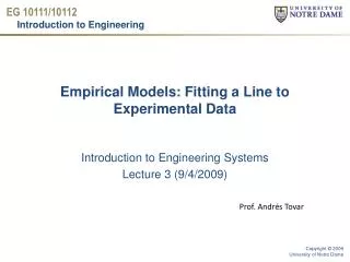
1. Empirical Models: Fitting a Line to Experimental Data Introduction to Engineering Systems Lecture 3 (9/4/2009) Prof. Andrés Tovar

2. Reading material and videos LC1 – Measure: Concourse material LT1 – Introduction: Sec. 1.1, 1.2, and 1.4 LT2 – Models: Ch. 4 LC2 – Matlab: Ch. 9 and 10, videos 1 to 9 LT3 – Data analysis: Sec. 5.1 to 5.3, videos 13 and 14 For next week LT4 – Statistics: Sec. 5.4.1 and 5.4.2, video 10 LC3 – SAP Model: Concourse material LT5 – Probability: Sec. 5.4.3 and 5.4.4, videos 11 and 12 LT: lecture session LC: learning center session Using "Laws of Nature" to Model a System

3. Announcements • Homework 1 • Available on Concourse http://concourse.nd.edu/ • Due next week at the beginning of the Learning Center session. • Learning Center • Do not bring earphones/headphones. • Do not bring your laptop. • Print and read the material before the session. Using "Laws of Nature" to Model a System

4. From last class pool ball golf ball • The 4 M paradigm: measure, model, modify, and make. • Empirical models vs. Theoretical models • Models for a falling object • Aristotle (Greece, 384 BC – 322 BC) • Galileo (Italy, 1564 – 1642) • Newton (England, 1643 – 1727) • Leibniz (Germany, 1646 –1716) • Models for colliding objects • Descartes (France, 1596-1650) • Huygens (Deutschland, 1629 – 1695) • Newton (England, 1643 – 1727) • Prediction based on models Empirical Models: Fitting a Line to Experimental Data

5. From last class pool ball golf ball • Given 2 pendulums with different masses, initially at rest • Say, a golf ball and a pool ball • Would you be willing to bet that you could figure out where to release the larger ball in order to knock the smaller ball to a given height? • How could you improve your chances? Empirical Models: Fitting a Line to Experimental Data

6. Theoretical Model of Colliding Pendulums pool ball golf ball • Given 2 pendulum masses m1 and m2 • golf ball initially at h2i = 0 • pool ball released from h1i • golf ball bounces up to h2f • pool ball continues up to h1f • Galileo’s relationship between height and speed later developed by Newton and Leibniz. • Huygens’ principle of relative velocity • Newton’s “patched up” version of Descartes’ conservation of motion—conservation of momentum Empirical Models: Fitting a Line to Experimental Data

7. Theoretical Model of Colliding Pendulums Collision model: Relative velocity Conservation of momentum Conservation of energy Conservation of energy Empirical Models: Fitting a Line to Experimental Data

8. Theoretical Model of Colliding Pendulums 1) Conservation of energy 2) Collision model: relative velocity and conservation of momentum 3) Conservation of energy Empirical Models: Fitting a Line to Experimental Data

9. Theoretical Model of Colliding Pendulums 4) Finally 4) In Matlab this is h1i = (h2f*(m1 + m2)^2)/(4*m1^2); Empirical Models: Fitting a Line to Experimental Data

10. Matlab implementation % collision.m m1 = input('Mass of the first (moving) ball m1: '); m2 = input('Mass of the second (static) ball m2: '); h2f = input('Desired final height for the second ball h2f: '); disp('The initial height for the first ball h1i is:') h1i = (h2f*(m1 + m2)^2)/(4*m1^2) Empirical Models: Fitting a Line to Experimental Data

11. Matlab implementation % collision1.m m1 = 0.165; % mass of pool ball, kg m2 = 0.048; % mass of golf ball, kg h2f = input('Desired final height for the second ball h2f: '); disp('The initial height for the first ball h1i is:') h1i = (h2f*(m1 + m2)^2)/(4*m1^2) plot(h2f,h1i,'o'); xlabel('h2f'); ylabel('h1i') hold on Let us compare the theoretical solution with the experimental result. What happened?!?! Empirical Models: Fitting a Line to Experimental Data

12. Run the Pendulum Experiment Empirical Models: Fitting a Line to Experimental Data

13. Experimental Results % collision2.m h1ie = 0:0.05:0.25; % heights for pool ball, m h2fe = []; % experimental results for golf ball, m plot(h1ie,h2fe,'*') Empirical Models: Fitting a Line to Experimental Data

14. MATLAB GUI for Least Squares Fit Empirical Models: Fitting a Line to Experimental Data

15. MATLAB commands for Least Squares Fit % collision2.m h1ie = 0:0.05:0.25; % heights for pool ball, m h2fe = []; % experimental results for golf ball, m plot(h1ie,h2fe,'*') c = polyfit(h1ie, h2fe, 1) m = c(1) % slope b = c(2) % intercept h2f = input('Desired final height for the second ball h2f: '); disp('The initial height for the first ball h1i is:') h1i = 1/m*(h2f-b) fit a line (not quadratic, etc) Empirical Models: Fitting a Line to Experimental Data

16. What About Our Theory Is it wrong? Understanding the difference between theory and empirical data leads to a better theory Evolution of theory leads to a better model Empirical Models: Fitting a Line to Experimental Data

17. Improved collision model Huygens’ principle of relative velocity Coefficient of restitution Improved collision model: COR and conservation of momentum The improved theoretical solution is hi1 = (h2f*(m1 + m2)^2)/(m1^2*(Cr + 1)^2) Empirical Models: Fitting a Line to Experimental Data

18. Matlab implementation % collision3.m m1 = 0.165; % mass of pool ball, kg m2 = 0.048; % mass of golf ball, kg Cr = input('Coefficient of restitution: '); h2f = input('Desired final height for the second ball h2f: '); disp('The initial height for the first ball h1i is:') hi1 = (h2f*(m1 + m2)^2)/(m1^2*(Cr + 1)^2) Let us compare the improved theoretical solution with the experimental result. What happened now? Empirical Models: Fitting a Line to Experimental Data