Download
1 / 40
420 likes | 712 Vues
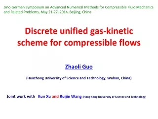
Sino-German Symposium on Advanced Numerical Methods for Compressible Fluid Mechanics and Related Problems, May 21-27, 2014, Beijing, China. Discrete unified gas-kinetic scheme for compressible flows. Zhaoli Guo (Huazhong University of Science and Technology, Wuhan, China)

E N D
Sino-German Symposium on Advanced Numerical Methods for Compressible Fluid Mechanics and Related Problems, May 21-27, 2014, Beijing, China Discrete unified gas-kinetic scheme for compressible flows Zhaoli Guo (Huazhong University of Science and Technology, Wuhan, China) Joint work with Kun Xu and Ruijie Wang (Hong Kong University of Science and Technology)
Outline • Motivation • Formulation and properties • Numerical results • Summary
Motivation Non-equilibrium flows covering different flow regimes Free-molecular Continuum Transition Slip 10-3 10-2 10-1 100 10 Re-Entry Vehicle Inhalable particles Chips
Challenges in numerical simulations Modern CFD: • Based on Navier-Stokes equations • Efficient for continuum flows • does not work for other regimes Particle Methods: (MD, DSMC… ) • Noise • Small time and cell size • Difficult for continuum flows / low-speed non-equilibrium flows Method based on extended hydrodynamic models : • Theoretical foundations • Numerical difficulties (Stability, boundary conditions, ……) • Limited to weak-nonequilibrium flows
= const Lockerby’s test (2005, Phys. Fluid) the most common high-order continuum equation sets (Grad’s 13 moment, Burnett, and super-Burnett equations ) cannot capture the Knudsen Layer, Variants of these equation families have, however, been proposed and some of them can qualitatively describe the Knudsen layer structure … the quantitative agreement with kinetic theory and DSMC data is only slight
MD NS A popular technique: hybrid method Limitations Numerical rather than physical Artifacts Time coupling Dynamic scale changes Hadjiconstantinou Int J Multiscale Comput Eng 3 189-202, 2004 Hybrid method is inappropriate for problems with dynamic scale changes
Efforts based on kinetic description of flows # Discrete Ordinate Method (DOM) [1,2]: • Time-splitting scheme for kinetic equations (similar with DSMC) • dt (time step) < (collision time) • dx (cell size) < (mean-free-path) • numerical dissipation dt Works well for highly non-equilibrium flows, but encounters difficult for continuum flows # Asymptotic preserving (AP) scheme [3,4]: • Consistent with the Chapman-Enskog representation in the continuum limit (Kn 0) • dt (time step) is not restricted by (collision time) • at least 2nd-order accuracy to reduce numerical dissipation [5] Aims to solve continuum flows, but may encounter difficulties for free molecular flows [1] J. Y. Yang and J. C. Huang, J. Comput. Phys. 120, 323 (1995) [2] A. N. Kudryavtsev and A. A. Shershnev, J. Sci. Comput. 57, 42 (2013). [3] S. Pieraccini and G. Puppo, J. Sci. Comput. 32, 1 (2007). [4] M. Bennoune, M. Lemo, and L. Mieussens, J. Comput. Phys. 227, 3781 (2008). [5] K. Xu and J.-C. Huang, J. Comput. Phys. 229, 7747 (2010)
Efforts based on kinetic description of flows # Unified Gas-Kinetic Scheme (UGKS) [1]: • Coupling of collision and transport in the evolution • Dynamicly changes from collision-less to continuum according to the local flow • The nice AP property A dynamic multi-scale scheme, efficient for multi-regime flows In this report, we will present an alternative kinetic scheme (Discrete Unified Gas-Kinetic Scheme), sharing many advantages of the UGKS method, but having some special features . [1] K. Xu and J.-C. Huang, J. Comput. Phys. 229, 7747 (2010)
Outline • Motivation • Formulation and properties • Numerical results • Summary
# Kinetic model (BGK-type) Distribution function Particel velocity Equilibrium: Flux Conserved variables Maxwell (standard BGK) Example: Shakhov model ES model
Conserved variables Conservation of the collision operator A property: for any linear combination of f and f eq , i.e., The conservation variables can be calculated by
# Formulation: A finite-volume scheme Trapezoidal Mid-point j+1/2 j j+1 Point 1: Updating rule for cell-center distribution function 1. integrating in cell j: 2. transformation: 3. update rule: Key: distribution function at cell interface
explicit Implicit j+1/2 So j j+1 Point 2: Evolution of the cell-interface distribution function How to determine Again Again 1. integrating along the characteristic line 2. transformation: Slope 3. original:
# Boundary condition n n Bounce-back Diffuse Scatting
# Properties of DUGKS 1. Multi-dimensional • It is not easy to device a wave-based multi-dimensional scheme based on hydrodynamic equations • In the DUGKS, the particle is tracked instead of wave in a natural way (followed by its trajectory) 2. Asymptotic Preserving (AP) (a) time step (t) is not limited by the particle collision time (): (b) in the continuum limit (t >> ): Chapman-Ensokg expansion in the free-molecule limit: (t << ): (c) second-order in time; space accuracy can be ensured by choosing linear or high-order reconstruction methods
# Comparison with UGKS j+1/2 j j+1 Unified GKS (Xu & Huang, JCP 2010) Starting Point: Macroscopic flux Updating rule: If the cell-interface distribution f(t) is known, the update bothfand W can be accomplished
Unified GKS (cont’d) j+1/2 j j+1 Key Point: Integral solution: Free transport Equilibrium After some algebraic, the above solution can be approximated as Chapman-Enskog expansion Free-transport
DUGKS vs UGKS • Common: • Finite-volume formulation; • AP property; • collision-transport coupling (b) Differences: in DUGKS • W are slave variables and are not required to update simultaneously with f • Using a discrete (characteristic) solution instead of integral solution in the construction of cell-interface distribution function
# Comparison with Finite-Volume LBM ci Lattice Boltzmann method (LBM) Standard LBM: time-splitting scheme Collision Free transport Evolution equation: Viscosity: Numerical viscosity is absorbed into the physical one Limitations: 1. Regular lattice 2. Low Mach incompressible flows
# Comparison with Finite-Volume LBM j+1/2 j j+1 Finite-volume LBM (Peng et al, PRE 1999; Succi et al, PCFD 2005; ) Micro-flux is reconstructed without considering collision effects Viscosity: Numerical dissipation cannot be absorbed Limitations(Succi, PCFD, 2005): 2. Large numerical dissipation 1. time step is limited by collision time Difference between DUGKS and FV-LBM: DUGKS is AP, but FV-LBM not
Outline • Motivation • Formulation and properties • Numerical results • Summary
Test cases • 1D shock wave structure • 1D shock tube • 2D cavity flow Collision model: Shakhov model
1D shock wave structure Parameters: Pr=2/3, = 5/3, Tw Left: Density and velocity profiles; Right: heat flux and stress (Ma=1.2)
DUGKS as a shock capturing scheme Density (Left) and Temperature (Right) profile with different grid resolutions (Ma=1.2, CFL=0.95)
1D shock tube problem Parameters: Pr=0.72, = 1.4, T0.5 Domain: 0 x 1; Mesh: 100 cell, uniform Discrete velocity : 200 uniform gird in [-10 10] Reference mean free path By changing the reference viscosity at left boundary, the flow can changes from continuum to free-molecular flows
2D Cavity Flow Domain: 0 x, y 1; Mesh: 60x60 cell, uniform Discrete velocity : 28x28 Gauss-Hermite Parameters: Pr=2/3, = 5/3, T0.81 Kn=0.075 Temperature. White and background: DSMC Black Dashed: DUGKS
Kn=0.075 Heat Flux
Kn=0.075 Velocity
UGKS: Huang, Xu, and Yu, CiCP 12 (2012) Present DUGKS Temperature and Heat Flux Kn=1.44e-3; Re=100
Comparison with LBM Stability: Re=1000 LBM becomes unstable on 64 x 64 uniform mesh UGKS is still stable on 20 x 20 uniform mesh 80 x 80 uniform mesh LBM becomes unstable as Re=1195 UGKS is still stable as Re=4000 (CFL=0.95)
Velocity DUGKS LBM
DUGKS LBM Pressure fields
Summary • The DUGKS method has the nice AP property • The DUGKS provides a potential tool for compressible flows in different regimes Thank you for your attention!