Introduction to Mad-X
270 likes | 493 Vues
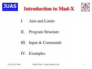
Introduction to Mad-X. Aim and Limits Program Structure Input & Commands Examples. Information. MAD-X webpage: http://mad.web.cern.ch/mad/ Or google search “madx cern” and use first entry. This seminar: http://cern.ch/Frank.Schmidt/Source/JUAS09-MADX (Talk, documentation and code)

Introduction to Mad-X
E N D
Presentation Transcript
Introduction to Mad-X Aim and Limits Program Structure Input & Commands Examples MAD-X Intro - Frank Schmidt, Cern
Information • MAD-X webpage: http://mad.web.cern.ch/mad/ • Or google search “madx cern” and use first entry. • This seminar: http://cern.ch/Frank.Schmidt/Source/JUAS09-MADX • (Talk, documentation and code) • MAD-X Primer: • http://cern.ch/Frank.Schmidt/report/mad_x_primer.pdf MAD-X Intro - Frank Schmidt, Cern
Description (+) • General optics design code for all sorts of accelerators and transfer lines. • The MAD input language has become a world standard. • MAD Machine descriptions can be found for many machines at many accelerator centers around the world • Powerful matching, correction and plotting algorithms. • Program Output comes in self-described table format that allows for easy post-processing with external analysis tools. • MAD-X is complemented by a more rigorous and object oriented code called PTC (beyond this introduction!) MAD-X Intro - Frank Schmidt, Cern
Description (-) • Main emphasis is optics and single particle dynamics. • Different codes needed for collective effects. • The code has been written in the early `80s (earliest reports from 1983 by Chris Iselin). Therefore the code comes with ancient programming structure with many modules written in Fortran77. • As a consequence • The code is fast • The results are not always consistent! • Main use for large machines and increasing problematic for small machines and when large chromatic effects become relevant. ( therefore PTC) • Do not use as a black box despite its reputation! (I will give an example) • In general the code is not really meant for beginners but rather made for accelerator experts. MAD-X Intro - Frank Schmidt, Cern
History & Code Features • To deal with the special case of the LHC, a double ring with common parts, a code MAD9 has been written but this code, despite its sophistication (C++, object oriented), was not fit for the job. • Therefore preparation of MAD-X, a re-write of the previous MAD8 version (pure Fortran77, still around but not maintained). • MAD-X: Core in C, modules in Fortran77, on Linux, Windows and Mac OS-X platforms. • Retain trustworthy parts of MAD8, more modular structure. New modules may be added in C or Fortran flavors. • Missing features recovered by complementing MAD-X with PTC. • Medium size code: MAD-X(110’000 lines) + PTC(100’000 lines Fortran90). • Code maintenance by a sizable group of module keepers (from various Labs) and one custodian. • Kept under CVS control. • Originally designed to serve the needs of LHC and presently prepared for a LHC online model. • All CERN machines and transfer lines beginning with the PS booster are kept as MAD-X input files (CAMIF CVS repository). • Plays also an essential role in the CLIC design, mainly using PTC. MAD-X Intro - Frank Schmidt, Cern
MAD-X Module Keepers • Catia Milardi (INFN/LNF) + Frank Zimmermann –Touschek • Etienne Forest (KEK) –Ptc proper • Frank Schmidt –Custodian,C6t, Twiss , Ptc, Linux • Frank Tecker –Survey • Frank Zimmermann –Dynap,IBS • Hans Grote –Core Maintenance & Debug • Helmut Burkhardt (Mark Hayes) –Makethin,Mac Version • Jean-Bernard Jeanneret –Aperture • Jean-LucNougaret – Ptc_twiss,Windows Version • Nikolay Malitsky (BNL) –Sxf • Riccardo de Maria (interim) –Match, Plot • Rogelio Tomás –Emit • Stefan Sorge (GSI) –Sodd • Thys Risselada –Threader • Valery Kapin (ITEP) –Ptc_track • Werner Herr –Error, Cororbit • Yipeng Sun –Thintrack MAD-X Intro - Frank Schmidt, Cern
Services • MAD-XWeb page: http://mad.web.cern.ch/mad/ • Documentation in HTML format derived from that source PS & PDF manual files. • Reports about MAD-X can be found at: http://mad.web.cern.ch/mad/reports/reference/node1.html In you find there the mad_x_primer.pdf • Link to the MAD-XExamples. In fact, for each new production version all examples will be rigorously checked for consistency with the results of the previous version. • News Section describing changes for each MAD-X production Version • Latest Executables for Linux, Windows, Mac. • Directory with SourceCode(files and tar),Makefiles & Project History. • MAD-XMailingList: You may subscribe to the MAD-X Mailinglist via an Email to hep-project-madx@cern.ch; in that Email put into the body the line: subscribe hep-project-madx@cern.ch After subscription you will receive a notification about new MAD-X production versions. • Pitfalls for beginners (even for experts!) should be read before first usage! MAD-X Intro - Frank Schmidt, Cern
Schematic Overview of MAD-X MAD-X Input Files Parser MAD-X Core C Conversion PTC Fortran90 Modules F77&C: Twiss Matching ThinTrack C6t … Modules F90: Ptc_twiss Parametric Matching Ptc_track Ptc_normal … TFS Table SixTrack: Fast Tracking Analysis MAD-X Intro - Frank Schmidt, Cern
Accelerator Design Work • Element Definition: • All standard linear accelerator elements (drifts, dipoles, quadrupoles, kickers). • Nonlinear elements (sextupoles, octupoles, multipoles). • “Special” elements (markers, rfcavities, electrostatic separators, solenoids, Beam-Beam elements). • Construction of an accelerator as a sequence of elements: • Placing elements at their longitudinal position s. • Misalignment of individual elements. • Defining free aperture for the beam in the elements. • Specifying linear and nonlinear imperfections. • Action commands: • Survey of the machine (global coordinates and check of closing of the machine). • Calculating the optical “Twiss” parameters, e.g. beta-functions, dispersion etc. • Global and local matching of Twiss parameters, tunes, linear coupling, chromaticities and others. • Orbit correction. • Particle tracking to find the “dynamic aperture”, i.e. the transverse oscillation amplitude beyond which single particle motion becomes unstable. MAD-X Intro - Frank Schmidt, Cern
MAD-X Input Language • Language similar to C, e.g. all statements must be terminated by “;” and a statement can go across any number of lines. • Comments: “!”, or “//” for the rest of the line or C constructs with start: “/*” and stop: “*/” key. • Besides the usual “=“ sign there is also “:=“ which allows to defer the evaluation to when it is needed, i.e. • a=b, a keeps its original value when b is changed. • a:=b, a obtains the new value of b when b is changed. • Variables of commands and elements can be accessed with the “->” operator • Complete C like pattern matching. • "if(){}", "else{}", "elseif(){}" statements. • “while(){}“ loop. • Powerful “macro” structures (beyond this introduction!). • Mathematical and physical constants, e.g. Pi, e, clight etc. (find all available constants at the top of the madxdict.h file). • System calls: system,”…”; beware of platform differences! MAD-X Intro - Frank Schmidt, Cern
Linear Elements A linear element is defined in the following way (I retain only the most relevant attributes – see MAD-X for full list and explanation): label: ELEMENT_TYPE, L=real, list_of_attributes…; • Drift: label: DRIFT, L=real; • Bend:a) label: SBEND, L=real, ANGLE=real, TILT=real, K1=real, E1=real, E2=real; b) label: RBEND, L=real, ANGLE=real, TILT=real, K1=real, E1=real, E2=real; • Quadrupole: label: QUADRUPOLE, L=real, K1=real, K1S=real, TILT=real; • Kicker (HKICKER & VKICKER exist also): label: KICKER, L=real, HKICK=real, VKICK=real, TILT=real; MAD-X Intro - Frank Schmidt, Cern
NonLinear Elements The nonlinear elements are defined in the following way: label: ELEMENT_TYPE, L=real, list_of_attributes…; • Sextupole: label: SEXTUPOLE, L=real, K2=real, K2S=real, TILT=real; lllllllll • Octupole: label: OCTUPOLE, L=real, K3=real, K3S=real, TILT=real; lllllllll • Multipole (zero-length kick L=0): label: MULTIPOLE, LRAD=real, TILT=real, KNL:={… , … , ...}, KSL:={… , ... , ...}; MAD-X Intro - Frank Schmidt, Cern
Strength Definition The strength definition of selected (non)linear elements: • Bend: ANGLE = L/(B ρ) By [rad] = L/ρ • Quadrupole: K1 = 1/(B ρ) ðBy /ðx [T/m] • Sextupole: K2 = 1/(B ρ) ð2By /ðx2 [T/m2] • Octupole: K3 = 1/(B ρ) ð3By /ðx3 [T/m3] MAD-X Intro - Frank Schmidt, Cern
Element Definition Example lq=3.0; lquad2:=1.5; lb:=2.0; // element definiton; mb: sbend, l:=lb, ANGLE=2.0*pi/320; qf: quadrupole, l=3.0, k1:=kqf; qf2: quadrupole, l=1.5, k1:=kqf; qd: quadrupole, l:=qf->l, k1:=kqd; ! use length of element qf qd2: quadrupole, l=1.5, k1:=qd->k1; ! use k1 of element qd kqf= 0.00197278; kqd=-0.0019508; ! Now non-linear elements lsx=1; ksx=0.01; sx1: sextupole, l=0, k2:=ksx; ! No effect acts like a marker sx2: sextupole, l:=lsx, k2:=ksx; ! sx2 sextupole with strength ksx ksx=0; ! Now the sx2 sextupole has no strength acts like a drift loc=1; koc=0.001; oc1: octupole, l:=loc, k3:=koc; ! oc1 octupole with strength koc m1: multipole, knl={0, 0, lsx*ksx}; ! m1 multipole with fixed sextupole strenght lsx*ksx /* m2 multipole with deferred skew quad, sext and oct strength kqn, ksn, kon */ m2: multipole, ksl:={0, kqn, ksn, kon}; MAD-X Intro - Frank Schmidt, Cern
Sequence Construction The elements are placed in a sequence that is defined as follows: name: SEQUENCE, REFER=keyword, REFPOS=name, LENGTH:=real label: class,AT=real{,attributes} | class,AT=real | sequ_name, AT=real ... ENDSEQUENCE • REFER is one of ENTRY, CENTER or EXIT. This attribute specifies the positioning with respect to AT. For CENTER (the default) the AT position is in the middle of the element. • AT is the absolute or relative position using FROM=name. • The LENGTH of the sequence has to be calculated. It can be a deferred variable. • In the body three types of commands can be placed: • A normal declaration of an element with an additional AT attribute. • A class with a position. • A sequence name with a position. The sequence is either placed with respect to the AT position and REFER or element as specified by the sequence attribute REPOS becomes the reference position. • There is no need to define drift they are generated automatically. • Beware: Defining an element twice in the same sequence is a fatal error! MAD-X Intro - Frank Schmidt, Cern
Sequence Example circum=200.0; ncell=5; lcell:=circum/ncell; //sequence declaration; JUAS_1a: sequence, refer = entry, l:=circum; start_machine: marker, at = 0; n=1; while (n<ncell+1) ! Notice neat use of the while loop { qf2: qf2, at=(n-1)*lcell; mb: mb, at=(n-1)*lcell+0.15*lcell; mb: mb, at=(n-1)*lcell+0.35*lcell; qd: qd, at=(n-1)*lcell+0.50*lcell-lquad2; mb: mb, at=(n-1)*lcell+0.65*lcell; mb: mb, at=(n-1)*lcell+0.85*lcell-lb; qf2: qf2, at=(n)*lcell-lquad2; n=n+1; value, n; ! Command value prints values, e.g. qf2->k1 } end_machine: marker, at = circum; endsequence; MAD-X Intro - Frank Schmidt, Cern
Action Commands • Most common action commands are TWISS and PLOT with a lot of options (see manual). • TWISS allows to calculate the standard Twiss but also user-defined parameters via the SELECT command. set, format="18.10e"; ! defines I/O precision ! suppress info, warning etc, actually not recommended! option, -info, -warn, verify, -echo; call, file="V6.5.seq"; call, file="V6.5.coll.str"; beam, sequence=lhcb1,particle=proton,energy=450; use, sequence=lhcb1; ! clear recommended since select is additive select, flag=twiss, clear; ! range to cut out the IR of all LHC select, flag=twiss, range=mqm.9l5.b1/mqm.9r5.b1, column=name,s,betx,bety,dx; twiss, sequence=lhcb1, file='twiss_lhc_ir'; ! range to cut out the IR of all LHC ! plot is without select ! interpolate calculates Twiss params within element plot,haxis=s, range=mqm.9l5.b1/mqm.9r5.b1, vaxis1=betx,bety,vaxis2=dx,colour=100,notitle, interpolate,file="lhc_ir"; MAD-X Intro - Frank Schmidt, Cern
TFS Example @ NAME %05s "TWISS“ TFS Header @ TYPE %05s "TWISS" @ SEQUENCE %05s "LHCB1" @ PARTICLE %06s "PROTON" @ MASS %le 9.3827201300e-01 @ CHARGE %le 1.0000000000e+00 @ ENERGY %le 4.5000000000e+02 @ PC %le 4.4999902183e+02 @ GAMMA %le 4.7960505457e+02 @ KBUNCH %le 1.0000000000e+00 … * NAME S BETX BETY DX TFS DATA $ %s %le %le %le %le "MQM.9L5.B1" 1.2988273212e+04 1.8297382970e+01 1.9697672117e+02 4.5339018235e-01 "DRIFT_34" 1.2988464212e+04 1.8446445353e+01 1.9521876944e+02 4.5024727875e-01 "MCBCV.9L5.B1" 1.2989364212e+04 1.9210419255e+01 1.8704627800e+02 4.3543778538e-01 "DRIFT_46" 1.2990346212e+04 2.0159915785e+01 1.7833820055e+02 4.1927898261e-01 "MCO.9L5.B1" 1.2990346212e+04 2.0159915785e+01 1.7833820055e+02 4.1927898261e-01 "DRIFT_164" 1.2990347712e+04 2.0161458665e+01 1.7832506585e+02 4.1925430012e-01 "MCD.9L5.B1" 1.2990347712e+04 2.0161458665e+01 1.7832506585e+02 4.1925430012e-01 "DRIFT_109" 1.2990681964e+04 2.0512305469e+01 1.7541088699e+02 4.1375417522e-01 "MB.B9L5.B1" 1.3004981964e+04 4.8646930598e+01 7.4404417008e+01 2.1490833470e-01 "DRIFT_110" 1.3005200717e+04 4.9276498079e+01 7.3218482234e+01 2.1242427713e-01 "MCS.B9L5.B1" 1.3005310717e+04 4.9595344783e+01 7.2626223621e+01 2.1117516617e-01 "DRIFT_111" 1.3006341470e+04 5.2656836237e+01 6.7209461158e+01 1.9947039863e-01 "MB.A9L5.B1" 1.3020641470e+04 1.0887728555e+02 1.6855184606e+01 7.3548999068e-02 "DRIFT_110" 1.3020860222e+04 1.0993645356e+02 1.6444096096e+01 7.2180527936e-02 "MCS.A9L5.B1" 1.3020970222e+04 1.1047132508e+02 1.6241469740e+01 7.1492390790e-02 "DRIFT_41" 1.3021794222e+04 1.1452626183e+02 1.4810656006e+01 6.6337617992e-02 "BPM.8L5.B1" 1.3021794222e+04 1.1452626183e+02 1.4810656006e+01 6.6337617992e-02 MAD-X Intro - Frank Schmidt, Cern
Triplet of the LHC (local matching) MAD-X Intro - Frank Schmidt, Cern
Global Match and Tracking !TITLE,'Thinless Tracking: Example chaos with particle loss'; beam, particle = proton, energy = 100; call file=fv9.opt; ! strength file sextupoles on call file="fv9.seq"; ! five cell sequence use,period=fivecell; ! make thin lattice for tracking makethin,sequence=fivecell; use,period=fivecell; twiss; ! undisturbed Twiss match, sequence=fivecell; vary, name=kqf, step=0.0001; vary, name=kqd, step=0.0001; ! The matching is supposed to go close to Q1=1/3 global, sequence=fivecell, Q1=1.333; global, sequence=fivecell, Q2=1.28; Lmdif, calls=50, tolerance=1.0e-6; endmatch; ! Twiss with hor tune close to 1/3 order resonance twiss; fac=2.0326; ! empircal factor to find chaos track,dump; start, x=fac*1e-2, px=0, y=30e-3, py=0; start, x=fac*2e-2, px=0, y=30e-3, py=0; start, x=fac*3e-2, px=0, y=30e-3, py=0; start, x=fac*4e-2, px=0, y=30e-3, py=0; start, x=fac*5e-2, px=0, y=30e-3, py=0; RUN, turns= 1793,ffile=1; ! particle lost turns > 1793 endtrack; plot, file="fv9_1_START",table=track,haxis=x,vaxis=px, particle=1,2,3,4,5, colour=1000, multiple, symbol=3; ! gnuplot "gnu_plot_my_lost.cmd" for optimal graphics MAD-X Intro - Frank Schmidt, Cern
Horizontal Phase Space MAD-X Intro - Frank Schmidt, Cern
Chromatic Problems of MAD-X • It is well known that treatment of chromatic effects is not optimal. • Moreover, it is a matrix code to second order. • Therefore, for very large relative momentum deviation δ= (p-p0)/p0we expect deviations from the correct results. • This has been pointed out to us several times e.g. a PAC2003 contribution (found in the documentation folder FPAG010.pdf): A COMPARISON OF SEVERAL LATTICE TOOLS FOR COMPUTATION OF ORBIT FUNCTIONS OF AN ACCELERATOR by Ernest D. Courant, Scott J. Berg Dejan Trbojevic and Richard Talman • The describe the physics of a cyclotron and give an analytical formula for the tune as a function of δ. • I have redone the calculation with MAD-X proper and also PTC. • The following graph shows the comparison. • The example shows one of the limits of MAD-X but that we can this handle these problems using more sophisticated tools. MAD-X Intro - Frank Schmidt, Cern
Simple Cyclotron MAD-X Intro - Frank Schmidt, Cern