Understanding Theoretical Probability Models: Binomial, Poisson, Exponential, and More
410 likes | 524 Vues
This module provides a comprehensive overview of key theoretical probability models, essential for decision analysis. It covers the Binomial, Poisson, Exponential, Normal, and Beta distributions, exploring their characteristics, mathematical formulations, and practical applications. Gain insights into frequent applications such as quality control, reliability, and survey sampling. The module also includes tutorials on the associated software, assisting in real-world problem-solving and decision-making by leveraging these probability distributions.

Understanding Theoretical Probability Models: Binomial, Poisson, Exponential, and More
E N D
Presentation Transcript
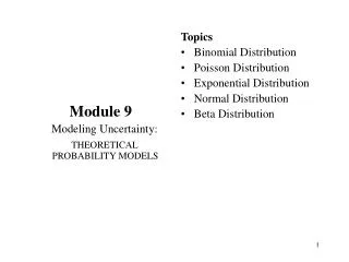
Module 9 Modeling Uncertainty: THEORETICAL PROBABILITY MODELS Topics Binomial Distribution Poisson Distribution Exponential Distribution Normal Distribution Beta Distribution
Introduction • Module 7: • basic probability • use in decision problems • Module 8: • subjective probability • modeling for decision analysis • Module 9: • theoretical distributions • application to decision analysis • Module 9 software tutorial
Theoretical Probability ModelsLearning Objectives • Refresh knowledge: • Binomial distribution • Poisson distribution • Exponential distribution • Normal distribution • Gain knowledge: • Beta distribution
Binomial Distribution(a discrete distribution) Model characteristics: • Dichotomous outcomes • Two possible outcomes • One outcome can occur • Constant probability of “success” • Independence
Binomial Distribution Mathematical model: • PB(R= r | n, p) = [n! / r! (n - r)!] pr(1-p)n-r • B subscript = binomial probability • R = binomial random variable • r = number of successful outcomes • n = number of events or trials • p = probability of successful outcome • E (R) = = np Var (R) = = np(1- p) • 2
Binomial Distribution Probability mass function notation: • f (x) = ( ) px qn-x • X = binomial random variable • x = number of successful outcomes • n = number of events or trials • p = probability of a successful outcome • q = 1 – p = probability of an unsuccessful outcome • E (X) = µ = np V (X) = σ2 = µq n x
Binomial Distribution Cumulative distribution function: • Probability of k or fewer “successful” outcomes • F (x ≤ k) = ∑ ( ) px qn-x k n x X = 0
Binomial Distribution • Frequent application situations: • Quality control • Reliability • Survey sampling • Approximation by other models: • Poisson: p → 0 and n → ∞ • Normal: p ≤ 0.5 and np > 5, OR p > 0.5 and nq > 5
Binomial Distribution Example application: Items are manufactured in large lots, from each of which twenty units are selected at random. The lot is accepted if the sample contains three or fewer defectives. If the production process yields, on the average, ten percent defectives, what is the probability of lot acceptance?
Binomial Distribution Formulation: Determine the probability of three or fewer “successes” in 20 independent trials, each having 0.1 probability of success. F (x ≤ 3) = ∑ ( ) (0.1)x (0.9)20-x = 0.867 3 20 x X = 0
Poisson Distribution(a discrete distribution) Model characteristics: • Time interval or spatial region • Probability of an event is small • Events are independent • Events take place at a constant rate
Poisson Distribution Mathematical model: • PP (X = k | m) = (e –m m k) / k ! • P subscript = Poisson probability • X = Poisson random variable • k = number of events that occur • e = natural logs base, 2.718… • m = mean number of event occurrences • E (X) = µ = m Var (X) = σ2 = m
Poisson Distribution Probability mass function notation: • f (x) = (e – λ λ x ) / x ! • x = number of event occurrences • λ = mean number of event occurrences • e = natural logs base, 2.718… • E (X) = µ = λ V (X) = σ2 = λ
Poisson Distribution Cumulative distribution function: • Probability of k or fewer occurrences within a temporal or spatial interval • F (x ≤ k) = ( e – λ λ x ) / x ! ∑ X = 0 k
Poisson Distribution • Frequent application situations: • Quality control • Reliability • Queuing • Physical properties • Approximation by another model: • Normal: λ > 5
Poisson Distribution Example application: The probability that a person will have a negative reaction to the injection of a certain serum is 0.001. Determine the probability that two or more of 1,000 people will have a negative reaction to the injection.
Poisson Distribution Formulation: Determine the probability that zero or one people will have a negative reaction when λ = np = 1, and take the complement. 1 – F (x ≤ 1) = 1 - e-11x / x! = 0.264 1 ∑ x= 0
Exponential Distribution(a continuous distribution) Model characteristics: • Time or distance between two outcome occurrences • Poisson model characteristics required • Uses Poisson mean ( m or λ )
Exponential Distribution Mathematical model: • f E ( T = t | m ) = me-mt • E subscript = exponential probability • T = exponential random variable • t = interarrival period • m = mean of Poisson distribution • e = natural logs base, 2.718.. • E (T) = μ = 1 / m Var (T) = σ2 = 1 / m2
Exponential Distribution Probability density function notation: • f (x) = λ e -λx • x = length of interval between occurrences • λ = mean of Poisson distribution • e = natural logs base, 2.718… • E (X) = μ = 1 / λ V (X) = σ2 = 1 / λ2
Exponential Distribution Cumulative distribution function: • Probability that the interval between two occurrences is of length k or less • F ( x ≤ k ) = ∫ λ e – λ x d x = 1 – e – λ k k 0
Exponential Distribution • Frequent application situations: • Quality control • Reliability • Queuing • Physical phenomena • Applicable when underlying process is Poisson
Exponential Distribution Example Application: The life of a certain brand of light bulb can be approximated by the exponential probability density function. If the mean life of the light bulb is 1,000 hours, determine the probability that the bulb will last more than 1,000 hours
Exponential Distribution Formulation: • Determine the probability that a light bulb will have a life of 1000 or fewer hours, when µ = 1000, and take the complement • µ = 1/λ = 1000 so λ = 1/1000 = 0.001 • 1 – F(x ≤ 1000) = 1 - ∫ 0.001 e-0.001x dx = 1 - {1- e-0.001(1000) } = 1 - {1 – e-1 } = 0.368 1000 0
Normal (Gaussian) Distribution(a continuous distribution) Model characteristics: • “Bell–shaped” curve • Effective for measured phenomena • Effective for multiple sources of uncertainty • Two parameters, µ and σ
Normal Distribution Mathematical model: • fn ( y | µ,σ2 ) = (2πσ2)-1/2 exp [ -(y-µ)2 / 2σ2] • N subscript = normal probability • y = value(s) of random variable Y • π = 3.14159… • e = natural logs base 2.718… • µ = the distribution mean • σ = the distribution standard deviation • E (Y) = µ Var (Y) = σ2
Normal Distribution Probability density function: • f (x) = (2πσ2)-1/2 exp [ -(x-µ)2 / 2σ2] - ∞ < x < ∞ - ∞ < µ < ∞ - σ > 0 - π, e are constants - µ, σ are parameters • E (X) = µ Var (X) = σ2
Normal Distribution Cumulative distribution function: • Probability that a value of x or less will occur • F (x) = (2πσ2)-1/2 ∫ exp [ -(v-µ)2 / 2σ2] dv • P (a < X ≤ b) = F (b) – F (a) = (2πσ2)-1/2∫ exp [ -(v-µ)2 / 2σ2] dv x -∞ b a
Normal Distribution • Frequent application situations: • measured phenomena • measured results of multiple additive phenomena • approximation of other distributions • numerous inferential statistical methods
Normal Distribution Example application: The ages of employees at a company are normally distributed with a mean of 50 years and a standard deviation of 5 years. Determine the percentage of employees whose ages are likely to be between 50 and 52.5 years.
Normal Distribution Formulation: • Determine the probability of age ≤ 50 years, and determine the probability of age ≤ 52.5 years. Take the difference, and multiply the result by 100 to obtain the percentage. • Using the standard normal variate, Z = (x –μ) / σ, and cumulative distribution function probabilities from either tabled values or appropriate software, we obtain F(x ≤ 50) = F(Z ≤ 0) = 0.5000 and F(x ≤ 52.5) = F(Z ≤ 0.5) = 0.6915 • Then P(50 < x ≤ 52.5) = 0.6915 – 0.5000 = 0.1915 or 19.15 %
Beta Distribution Model characteristics: • Variable bounded at both ends • Numerous distribution shapes • Events are independent • Models proportions
Beta Distribution Generalized beta probability density function: • f (x | λ1, λ2, ω1, ω2) = where - ω1 ≤ x ≤ ω2 - λ1, λ2, ≥ 0 - Γ(λ) = (λ – 1)! when λ Є I+, OR ( ) ( ) λ2-1 1 λ1-1 (λ1+λ2) Γ ____ _________ ______ x – ω1 _____ x – ω1 1 - ω2 – ω1 ω2 – ω1 ω2-ω1 Γ (λ1) Γ (λ2) ∞ = ∫ xλ-1 e-x dx otherwise 0
Beta Distribution More frequently, set ω1 = 0 and ω2 =1 • So f (x | λ1, λ2) = xλ1-1 (1-x)λ2-1 Where 0 ≤ x ≤ 1 λ1, λ2 ≥ 0 Γ (λ) = (λ-1)! Where λ Є I+, OR = __________ Γ (λ1+ λ2) Γ (λ1) Γ (λ2) ∞ ∫ xλ-1 e-x dx otherwise 0
Beta Distribution • When λ1 and λ2 are positive integers: • Probability density function f (x | λ1,λ2) = x λ1-1 (1 – x)λ2-1 where the random variable X = x and 0 ≤ x ≤ 1 (λ1+ λ2 – 1)! _____________ (λ1 – 1)! (λ2 – 1)!
Beta Distribution • Let n = λ1 + λ2 and r =λ1 • f β ( q | r,n ) = q r-1( 1 – q )n-r-1 • β subscript = beta probability • Q = Beta random variable • q = proportion value between 0 and 1 • r = number of “successes” • n = number of trials • E (Q) = µ = r / n Var (Q) = σ2 = r ( n – r) / [ n2 ( n + 1) ] ________________ (n – 1)! ( r – 1) ! ( n – r – 1) !
Beta Distribution Cumulative distribution function: • F (Q ≤ q | r,n) = ∫ υr-1 (1 – υ) dυ • Called Incomplete Beta Function • Equivalence to binomial cumulative distribution function • Values from tables or software ______________ (n – 1)! q (r – 1)! (n – r – 1) 0
Beta Distribution • Frequent application situations: • Proportions or percentages • Physical variables in restricted intervals • Tolerances in quality control and reliability • PERT networks (generalized form) • Bayesian analysis (informative a priori) • Approximated by difference between two normal distributions when λ1+λ2 ≥ ~ 30
Beta Distribution Example Application: • Suppose that the percentage of employees who submit medical benefits claims each year is a beta random variable. As the benefits coordinator for a small firm with 40 employees, you currently expect that about 30 percent will most likely submit claims this year. Determine the probability that more than 16 employees will submit claims.
Beta Distribution Formulation: • Determine the probability that 16 or fewer of 40 employees will submit claims, and take the complement. • μ = r/n = 0.30 = r = (0.30)(40) = 12 q = 16/40 = 0.40 • From table values or software, Fβ (Q ≤ 0.40 | 12, 40) = 0.91 • Thus Pβ (Q > 0.40) = 1 – 0.91 = 0.09
Summary • Theoretical distributions to model uncertainty • Five distributions: • Binomial • Poisson • Exponential • Normal • Beta • Each distribution: • Mathematical formulation • Mean and variance • Graphical representations • Application situations • Example problem
