Download
1 / 50
500 likes | 500 Vues
This research study analyzes the formation of defects in convective patterns using the Regularized Cross-Newell Phase Diffusion Equation. The study explores the behavior of wave vectors and their variations in space and time, as well as the impact of twist on the patterns. The results are compared with experimental and numerical data.

E N D
Defect Formation in Convective Patterns as seen from the Regularized Cross-Newell Phase Diffusion Equation R. Indik, A.C. Newell, S. Venkataramani (Arizona) T. Passot (Nice) M. Taylor (UNC Chapel Hill) The Geometry of the Phase Diffusion Equation, J. Nonlinear Sci. 10, 223-274 (2000) Global Description of Patterns Far From Onset: A Case Study PhysicaD 184, 127-140 (2003)
Patterns far from threshold • In an isotropic stripe pattern-forming system, the direction of the wavevector is not chosen. Such structures can then be described by noting that the pattern locally consists of patches with a preferred wavevector k. One can then let kvary slowly in space and time • Experiment: From Y.-C. Hu, R. Ecke, & G. Ahlers, Phys. Rev. E 51, 3263 (1995). See also • http://tweedledee.ucsb.edu/~guenter/picturepage2.html
Convex Disclination Pr = 1.4 v.d.t.=2s courtesy of Eberhard Bodenschatz
Concave Disclination Aspect ratio = 30 Pr = 0.32 Courtesy of G. Ahlers, U.C. Santa Barbara http://tweedledee.ucsb.edu/~guenter/picturepage5.html
Outline I. Without Twist A. Motivation B. Swift-Hohenberg Model C. Cross-Newell Equation D. Regularization E. Results F. Self-Duality II. With Twist A. Director Fields B. Energetics C. Comparisons (Numerical and Experimental) D. Rigorous Scaling for Extended CN system
Swift-Hohenberg Swift-Hohenberg Eqn: ut = - (kc+D)2 u + m u – u3 SH Energy Density: - ½ ((kc+D)u)2 + ½ m u2 – ¼ u4 Family of Exact Stationary Solutions: u0(x) = a1(k) cos(q) + a2(k)cos(2q) + … k u0 = const. 2p/k
Cross – Newell Equation • Slowly Varying Rolls Modulational Ansatz • u = ue (Q/e) Q = Q (X,Y,T)Q = k(X,Y,T) k = |k| • Q = e qX= e x Y =e yT = e2 t t(k2)Q T = - ·(k B(k2)) • M.C. Cross & A.C. Newell, Convection patterns large aspect ratio systems, • Physica 10 D, 299-328 (1984)
Cross-Newell Energy Densityt(k2)Q T = - ·(k B(k2)) t(k2) (kc = kB = 1) kB(k2)
Regularized Cross-Newell Eqn t(k2) QT = - (k B(k2) + e2 D k) QT =k~1 - (2 Q (1 – |Q|2) ) - e2 D D Q) RCN Energy: Fe (Q) = e(DQ)2 +1/e (1-|Q|2)2dX dY
Regularized CN Disclinations C. Bowman
Analytical Results • Fe (Q) = e(DQ)2 +1/e (1-|Q|2)2dX dY • As e 0, minimizers Qe Q0 in H1(W)where Q0 solves • the eikonal equation |Q0| = 1. Defects are, therefore, • supported on locally 1-dimensional sets. An example of an • eikonal solution on a domain W: Q0 (x) = dist (x , W ). • (2) There is a natural conjecture that the asymptotic value of • the minimal energy (ground state energy) = a “jump energy” • supported on the defect locus S : • lim infe 0 1/3 |[Q0]|3 ds • where [Q0] = jump in k0 across S.
Eikonal Viscosity Solutions N=32 q N=32 q
(3) The conjecture can be completely verified in the class of examples where S is a straight line segment. In this same class the asymptotic energy is supported only on the 1-dimensional eikonal defects. Lower dimensional singularities carry no energy. • Ambrosio, DeLellis, Mantegazza • DeSimone, Kohn, Müller, Otto • Ercolani, Taylor
Analytical Difficulties of RCN: 1) 4th order (QT = - (2 Q (1 – |Q|2) ) - e2 D D Q) 2) Hausdorff dim of defects is > 0 (not point defects) Self-Dual Eqn:e(DQ) = (1-|Q|2) 1) Motivated by equi-partition of energy e(DQ)2 +1/e (1-|Q|2)2 2) If the Gaussian curvature of the graph of QSD vanishes, then QSD solves RCN 3) In the e-> 0 limit, the curvature of QSD concentrates in points.
Helmholtz Linearization • The substitution Q = e ln Y reduces • e(DQ) (1-|Q|2) = 0 • to the linear Helmholtz eqn: • e2DY - Y = 0
Self-Dual Test Functions Thm: Suppose ve solves e(D ve)+(1-| ve|2) = 0 on W with ve = q on the boundary of W where |q(x) - q(y)| a dist(x,y) with a < 1. Then as e 0, ve converges uniformly on the closure of W to the unique viscosity solution of | v|2 - 1 = 0 on W with v = q on W.
Steepest Descent These conditions are equivalent to k satisfying the jump conditions for a weak solution of stationary CN.
Outline I. Without Twist A. Motivation B. Swift-Hohenberg Model C. Cross-Newell Equation D. Regularization E. Results F. Self-Duality II. With Twist A. Director Fields B. Energetics C. Comparisons (Numerical and Experimental) D. Rigorous Scaling for Extended CN system
Boussinesq Simulation courtesy of Mark Paul b/a = 1.9 e = 0.850
Swift-Hohenberg equation q q N=32 N=32 m= 0.5, b/a = 1.9 e = 0.850
Comparison of knee solution to concave-convex disclination pair 8/3 sin3(a) 8/3 (1 - sin (a)) Energy cost per unit length of GB
Phase Topology • u() ~ cos() • k = = (f,g) Target Space Identifications: • + 2n • (,f,g) (-,-f,-g) Quotient map has critical points at = n; i.e., d = f dx + g dy behaves like a quadratic differential
Knee-to-Disclination Pair Transition Triangle: curvature center Diamond: critical transition
Fluid Experiment b/a = 1.5 Courtesy of G. Ahlers and W. Meevasana U.C.S.B.
Comparison with Other Simulations Swift-Hohenberg simulation Boussinesq simulation
Cross-Newell Zippers • cos((x,y)) is even in y and smooth in (x,y) (x,y) is an even function of y y (x,0) = 0; or, (x,y) is an odd function of y modulo • x cos() as y • Shift-periodic symmetry in x: (x+l ,y) = (x,y) + where l = cos()
Boundary Conditions • (x,0) = 0 for 0 x a • y(x,0) = 0 for a x l • (x+l ,y) = (x,y) + • xcos() + ysin() + • as y • Domain is S (boxed strip) • = cos()
Rigorous Scaling Law for Energy Minimizers • Natural small parameter here is = cos()