Image Compression: Coding and Decoding
This course segment provides a comprehensive introduction to image compression methods within digital image processing. It covers fundamental concepts of image encoding and decoding, highlighting the importance of redundancy removal in compression. Key topics include entropy and entropy coding, compression ratios, lossless vs. lossy compression, and practical examples such as Run-Length Coding and Variable Word Length Coding. By understanding these techniques, students will gain insight into how images can be efficiently stored and transmitted while maintaining quality.

Image Compression: Coding and Decoding
E N D
Presentation Transcript
EE4328, Section 005 Introduction to Digital Image ProcessingImage CompressionZhou WangDept. of Electrical EngineeringThe Univ. of Texas at ArlingtonFall 2006
Image Compression: Coding and Decoding original image 262144 Bytes From [Gonzalez & Woods] From [Gonzalez & Woods] compressed bitstream 00111000001001101… (2428 Bytes) image encoder image decoder compression ratio (CR) = 108:1
Some General Concepts • How Can an Image be Compressed, AT ALL!? • If images are random matrices, better not to try any compression • Image pixels are highly correlated redundant information • Information, Uncertainty and Redundancy • Information is uncertainty (to be) resolved • Redundancy is repetition of the information we have • Compression is about removing redundancy because • Entropy and Entropy Coding • Entropy is a statistical measure of uncertainty, or a measure of the amount of information to be resolved • Entropy coding: approaching the entropy (no-redundancy) limit
More Concepts • Bit Rate and Compression Ratio • Bit rate: bits/pixel, sometimes written as bpp • Compression ratio (CR): • Binary, Gray-Scale, Color Image Compression • Original binary image: 1 bit/pixel • Original gray-scale image: typically 8bits/pixel • Original Color image: typically 24bits/pixel • Lossless, Nearly lossless and Lossy Compression • Lossless: original image can be exactly reconstructed • Nearly lossless: reconstructed image nearly (visually) lossless • Lossy: reconstructed image with loss of quality (but higher CR) number of bits to represent the original image CR = number of bits in compressed bit stream
Run Length Coding • Run Length • The length of consecutively identical symbols • Run length Coding Example • When Does it Work? • Images containing many runs of 1’s and 0’s • When Does it Not Work?
Run Length Coding CCITT test image No. 1 Size: 17282376 1 bit/pixel (bpp) original: 513216 bytes compressed: 37588 bytes CR = 13.65
Run Length Coding • Decoding Example A binary image is encoded using run length code row by row, with “0” represents white, and “1” represents black. The code is given by Row 1: “0”, 16 Row 2: “0”, 16 Row 3: “0”, 7, 2, 7 Row 4: “0”, 4, 8, 4 Row 5: “0”, 3, 2, 6, 3, 2 Row 6: “0”, 2, 2, 8, 2, 2 Row 7: “0”, 2, 1, 10, 1, 2 Row 8: “1”, 3, 10, 3 Row 9: “1”, 3, 10, 3 Row 10: “0”, 2, 1, 10, 1, 2 Row 11: “0”, 2, 2, 8, 2, 2 Row 12: “0”, 3, 2, 6, 3, 2 Row 13: “0”, 4, 8, 4 Row 14: “0”, 7, 2, 7 Row 15: “0”, 16 Row 16: “0”, 16 decode Decode the image
Run Length Coding • Decoding Example A binary image is encoded using run length code row by row, with “0” represents white, and “1” represents black. The code is given by Row 1: “0”, 16 Row 2: “0”, 16 Row 3: “0”, 7, 2, 7 Row 4: “0”, 4, 8, 4 Row 5: “0”, 3, 2, 6, 3, 2 Row 6: “0”, 2, 2, 8, 2, 2 Row 7: “0”, 2, 1, 10, 1, 2 Row 8: “1”, 3, 10, 3 Row 9: “1”, 3, 10, 3 Row 10: “0”, 2, 1, 10, 1, 2 Row 11: “0”, 2, 2, 8, 2, 2 Row 12: “0”, 3, 2, 6, 3, 2 Row 13: “0”, 4, 8, 4 Row 14: “0”, 7, 2, 7 Row 15: “0”, 16 Row 16: “0”, 16 decode
contour image region image n m Chain Coding Assume the image contains only single-pixel-wide contours, like this, not this From Prof. Al Bovik After the initial point position, code direction only (3bits/step) Code Stream: (3, 2), 1, 0, 1, 1, 1, 1, 3, 3, 3, 4, 4, 5, 4 initial point position chain code
Chain Coding • Decoding Example The chain code for a 8x8 binary image is given by: column row (1, 6), 7, 7, 0, 1, 1, 3, 3, 3, 1, 1, 0, 7, 7 decode Decode the image
Chain Coding • Decoding Example The chain code for a 8x8 binary image is given by: column row (1, 6), 7, 7, 0, 1, 1, 3, 3, 3, 1, 1, 0, 7, 7 decode
Variable Word Length Coding • Intuitive Idea • Assign short words to gray levels that occur frequently • Assign long words to gray levels that occur infrequently • How Much Can Be Compressed? • Theoretical limit: entropy of the histogram • Practical algorithms (approach entropy): Huffman coding, arithmetic coding Maximum entropy: Uniform distribution typically in-between Minimum entropy: Impulse (delta) distribution From Prof. Al Bovik
Variable Word Length Coding: Example • A 4x4 4bits/pixel original image is given by Default Code Book 0: 0000 1: 0001 2: 0010 3: 0011 4: 0100 5: 0101 6: 0110 7: 0111 8: 1000 9: 1001 10: 1010 11: 1011 12: 1100 13: 1101 14: 1110 15: 1111 Bit rate = 4bits/pixel Total # of bits used to represent the image: 4x16 = 64 bits encode
Variable Word Length Coding: Example • Encode the original image with a CODE BOOK given left Huffman Code Book 0: 0000000 1: 0000001 2: 0001 3: 0000010 4: 0000011 5: 0000100 6: 01 7: 0000101 8: 10 9: 00100 10: 11 11: 0000110 12: 0000111 13: 001010 14: 0011 15: 001011 Total # of bits used to represent the image: 4+2+2+2+2+2+2+2+2+2+2+2+5+2+2+4 = 39 bits encode Bit rate = 39/16 = 2.4375 bits/pixel CR = 64/39 = 1.6410
image histogram (high entropy) DPCM histogram (low entropy) Predictive Coding • Intuitive Idea • Image pixels are highly correlated (dependent) • Predict the image pixels to be coded from those already coded • Differential Pulse-Code Modulation (DPCM) • Simplest form: code the difference between pixels • Key features: Invertible, and lower entropy (why?) DPCM: 82, 1, 3, 2, -32, -1, 1, 4, -2, -3, -5, …… Original pixels: 82, 83, 86, 88, 56, 55, 56, 60, 58, 55, 50, …… From Prof. Al Bovik
Advanced Predictive Coding • Higher Order (Pattern) Prediction • Use both 1D and 2D patterns for prediction • Apply Image Transforms before Predictive Coding • Decouple dependencies between image pixels • Use Advanced Statistical Image Models • Better understanding of “the nature” of image structures implies potentials of better prediction 1D Causal: 2D Causal: 1D Non-causal: 2D Non-Causal:
Quantization • Quantization: Widely Used in Lossy Compression • Represent certain image components with fewer bits (compression) • With unavoidable distortions (lossy) • Quantizer Design • Find the best tradeoff between maximal compression minimal distortion • Scalar Quantization Uniform scalar quantization: 248 8 40 ... 24 1 2 3 4 Non-uniform scalar quantization:
Quantization • Vector Quantization • Group multiple image components together form a vector • Quantize the vector in a higher dimensional space • More efficient than scalar quantization (in terms of compression) image component 2 Vector quantization: image component 1 From Prof. Al Bovik
Ideas on Lossy Image Compression code each block independently • Block-Based Image Compression • Transform-Domain Compression • Scalar or vector quantization of transform coefficients (instead of image pixels) Partition image From Prof. Al Bovik
Discrete Cosine Transform (DCT) • 2D-DCT: • Inverse 2D-DCT: where discontinuities: high frequencies continuous • DFT vs. DCT periodic extension by DFT reflected periodic extension by DFT From Prof. Al Bovik
2D-DCT image block DC component low frequency high frequency 2D-DCT low frequency high frequency DCT block
JPEG Compression • Partition the image into 8x8 blocks, for each block - 128 DCT scalar quantization zig-zag scan
JPEG Compression • Adjust Quantization Step to Achieve Tradeoff between CR and distortion JPEG: 5KB Original: 100KB JPEG: 9KB • Artifacts: Inside blocks: blurring (why?); Across blocks: blocking (why?)
Wavelet and JPEG2000 Compression • Wavelet Transform Energy Compaction Lower Entropy
Wavelet and JPEG2000 Compression • Bitplane Coding • Scan bitplanes from MSB to LSB • Progressive (scalable) JPEG2000 (64:1) JPEG (64:1)