Chapter 5 Exponential and Logarithm Functions
Chapter 5 Exponential and Logarithm Functions. Do Now!!! . Sketch the graphs of on the same coordinate plane. Compare the two graphs. Solution:. the graphs are both increasing the graphs both intersect the point (0,1)

Chapter 5 Exponential and Logarithm Functions
E N D
Presentation Transcript
Chapter 5 Exponential and Logarithm Functions
Do Now!!! Sketch the graphs of on the same coordinate plane. Compare the two graphs. Solution: • the graphs are both increasing • the graphs both intersect the point (0,1) • the graphs both have a horizontal asymptote at y = 0 • the graph with base 5 is steeper than the graph with base 2.
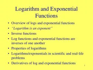
Lesson 5.1: Introduction One of the first topics discussed in Algebra concerns the Laws of exponents. However, our exponent was not the variable. This section will have our variable be the exponent. When the exponent is the variable our output converges upon some value called a Limit. Again, we have used an intuitive notion of “approaching” which is made Precise in calculus with the concept of the LIMIT.
5.2 The Natural Exponential Function Exponential functions have the form where a ≠ 1, the base, whose domain is the set of all real numbers. Below are some examples for a > 1. Notice that all have a horizontal asymptote at y = 0.
Once the graph of for a > 1, is known, the graph of its reciprocal can be found. Reciprocal of an exponential function Since, 1 < a Exponential function The reciprocal of a is always a value between 0 and 1 if the original exponential function has a > 1; it too will have a horizontal asymptote at y = 0.
Summary: • If a > 1, graph will increase • the larger the value of a the steeper the graph • Horizontal asymptote at y = 0 • Intersects the y-axis at (0, 1) • If 0 < a < 1, the graph will decrease • The larger the value of a, the wider the graph (closer to the x-axis) • Horizontal asymptote at y = 0 • Intersects the y-axis at (0,1)
example: Use the graph of to sketch the graph of We can see that the domain of f is (-∞, ∞), the range is (-3, ∞) and the graph has y = -3 as a horizontal asymptote.
To obtain this graph we need to vertically stretch the graph of by a • factor of 3, then shift it one unit to the right, reflect it over the x – axis and then • shift it one unit up.
Each exponential function can be converted to a scaled function of any single exponential function simply by letting a be raised to some power, then raised to the power of x. There is always some value where: Note: the value of 2 is simply an arbitrary value. Any positive value may be used, except, a ≠ 1 Natural Exponential Function: The number chosen for the natural exponential function is the irrational number denoted by the letter e. e ≈ 2.718
Since e is between 2 and 3, lies between example: Sketch the graph of The graph is obtained by translating the graph of to the right one unit, reflecting it over the x-axis and then shifting it up 2 units. Note: the graph now has a horizontal asymptote at y = 2.
example: Sketch the graph of You first must note that is simply a reflection about the y-axis of the graph Q: Reflecting about the y-axis yields a graph that is doing what? A: Decreasing. This is similar to 0 < a < 1; reciprocals. When we look at f(x) this is the arithmetic combination of functions. We are adding the output of two separate graphs over the same domain.
example: Approximate the value of k for which This is an arbitrary exponential function being turned into a scaled natural exponential function. We cannot yet determine the exact value of the constant needed to change this, but we can use a graphing device to find a close approximation. solution: By letting x = 1, we can eliminate this from our problem. We now have We now need to find the value of k that will make this statement true. Lets graph y = 2 and on the same coordinate plane. We can see that intersects y = 2 at about 0.7. If we zoom in on that intersection we can see that it is approximately 0.69, so are equal when k = 0.69, therefore, yielding the same graph.
example: Sketch the graph of Solution: • As x becomes large f(x) approaches 0 • rapidly • Since f(-x) = f(x) it has y-axis symmetry • and passes through (0,1) • We can see that the graph has the • appearance of a bell-shaped curve which is • associated with the normal distribution in • statistics
Compounding Interest Suppose we want to invest a sum of money into an interest bearing account. The Amount in the account at the end of t years depends on the interest rate and on The number of times the interest is compounded The greater the number of times the account is compounded the greater the Amount that will be in the account at the end of t years. The best possible of all situations is when the interest is compounded continuously. Standard form of equation for compounding interest: continuously
Annually: n = 1 Semi annually: n = 2 Quarterly: n = 4 Monthly: n = 12 Weekly: n = 52 Daily: n = 365 Hourly: n = 8760 Minutely: n = 525,600 example: Determine the value of a CD in the amount of $1000 that matures in 6 years and pays 5% per year compounded annually, monthly, daily, and continuously.
example: Determine the approximate length of time it takes an amount to double in value if it earns 9% compounded daily. solution: We do not know the value of our principle, so we simply leave in our variable. Since we do not know how to solve for variables in the power (yet ) we will use a graphing device and assume that we are compounding continuously instead of daily. We do this because it will be a result that is very close to the correct answer and it will look like an equation we already have worked with. Graph both equations in the same coordinate plane and see where they intersect. We find that they intersect around x = 7.7 years