Eikonal Equation
Eikonal Equation. k + k = 1. 2. 2. x. z. w. w. c. Plane wave (local homogeneous). 2. 2. 2. Apparent velocity. T + T = 1. 2. 2. c. 2. t(x,z)=2. z. t(x,z)=1. x. 2. 2. 2. (dt/dx) + (dt/dz) = (1/c). Eikonal Eqn. Eikonal Equation. k + k = w. 2. 2.

Eikonal Equation
E N D
Presentation Transcript
k + k = 1 2 2 x z w w c Plane wave (local homogeneous) 2 2 2 Apparent velocity T + T = 1 2 2 c 2 t(x,z)=2 z t(x,z)=1 x 2 2 2 (dt/dx) + (dt/dz) = (1/c) Eikonal Eqn. Eikonal Equation k + k = w 2 2 2 Dispersion Eqn. x z c 2 High freq. approx.
FD Soln of Eikonal Equation Step 1. Solve for times around src pt. by t=dr/c Times dr/c dr/c
2 2 2 (dt/dx) + (dt/dz) = (1/c) 2 (Ta – Tb) 2 2 2 (Ta – Tb) + (Tc-Td) = s s - 2 2 Td = Tc - 4dx 4dx 4dx 4dx 2 2 2 d a b c FD Soln of Eikonal Equation Step 2. Solve for times around next grid by FD dx
d b c FD Soln of Eikonal Equation Step 2. Solve for times around next grid by FD 2 2 2 (dt/dx) + (dt/dz) = (1/c) 2 2 2 (Ta – Tb) + (Tc-Td) = s 2dx 2dx 2 2 a dx
FD Soln of Eikonal Equation Step 3. Solve for times around next grid by FD 2 2 2 (dt/dx) + (dt/dz) = (1/c) 2 2 2 (Ta – Tb) + (Tc-Td) = s 2dx 2dx 2 2
FD Soln of Eikonal Equation Step 4. Repeat 2 2 2 (dt/dx) + (dt/dz) = (1/c)
Summary • Compute traveltime fields t(x,z) for each • Src. By a FD soln of Eikonal eqn. 2. t(x,z) used for traveltime tomography and migration. 3. First arrival energy not most energetic. Warning for migrationists. 4. First arrival energy for tomographers.
T(x+dx) dx along ray dx = T ds Distance along ray T(x) x x+dx c T =1 Eikonal eqn. says Ray Tracing c (1) Desire to eliminate T dependency in eq. 1
T(x+dx) ( ) dx = T c ds = T = c T ( ) T(x) dx ( ) ds d d 2 -2 = c ( ) T = c ( ) c = c - T ds ds c 2 2 2 Ray Tracing
T(x+dx) ( ) F(x) T(x) d d = = c c or 1st-order ODE’s - - ds ds dx c c 2 2 = F(x) c ds 0th-Order Shooting Ray Tracing ( ) dx c ds Specify start pt and direction 3 coupled 2nd-order ODE’s
Beware Caustics: zero area, phase change x 0th-Order Shooting Ray Tracing Green’s Function 1. Shoot two neighboring rays from x’. 2. Measure area A(x|x’) at x x’ 3. G(x’|x) = W(t-T )/A(x|x’) A(x|x’)
Interpolation Interpolation Summary • Compute traveltime fields t(x,z) for each • Src. By a FD soln of Ray Equations. 2. t(x,z) used for traveltime tomography and migration. 3. Good for migration, avoid head waves. 3. Does not accurately handle caustics. Higher-order ray theory needed such as Maslov or Gaussian Beam.
Transmission Reflection A B x B * T = min(T + T ) * T = min(T ) AB Ax xB AB AB rays rays Fermat’s Principle • Stationary ray between two points is shortest traveltime ray = specular ray. (i.e., Snell’s law) A
Fermat’s Principle • Stationary ray between two points is shortest traveltime ray = specular ray. Multiple Reflection A B x’ x * T = ????????????????? AB