Download
1 / 27
270 likes | 380 Vues
This comprehensive guide explores key concepts in managerial accounting, focusing on Cost-Volume-Profit (CVP) analysis and budgeting. Learn to forecast costs based on fixed and variable cost patterns, break-even analysis, and the significance of contribution margins. The guide covers estimating costs using the high-low method, segment reporting, and standard costs while introducing capital budgeting concepts such as Net Present Value (NPV) and Internal Rate of Return (IRR). Gain insights into effective financial decision-making and learn how to develop a master budget for your organization.

E N D
ManagerialAccounting Week 5 Notes David B. Hamm, MBA, CPA June, 2002 Revised Nov. 2003 & June 2004
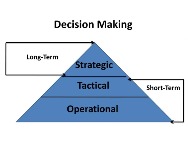
Cost-Volume-Profit Analysis (1) • Because of the unique patterns of fixed and variable costs, we can use these patterns to assist us in forecasting costs and planning optimal production activities. • This can be done graphically by plotting FC and VC for various production levels, or can be done with simple algebra • Break even costs: S = VC + FC where S=PxQ and VC=Cost x Q
C-V-P Analysis (2) • Illustration: Selling price= $10 per unit, VC=$6 per unit, and FC=$100,000. What is break even sales level? • Formula 10q = 6q + 100,000 • Thus: 4q = 100,000 (contribution margin is S – VC or $4 per unit) • q = 25,000 units (to break even)
C-V-P Analysis (3) • Suppose we desire a $2 profit per unit? Just add to the formula: • Sales = VC + FC + Profit, or • 10q = 6q + 100,000 + 2q • 2q = 100,000 • q = 50,000 units required sales to make a $2 profit per unit sold
Estimating Costs: High-Low • Previous data assumed FC and VC were easily obtained, but what if costs are “mixed”—elements of both fixed and variable costs combined? • Linear regression—most accurate method to break out costs • High-Low: quick method to estimate variable and fixed cost portions
High-Low: Illustration (1) There is a clear relationship between quantity and cost, but it is not yet specified
High-Low: Illustration (2) Thus VC estimated = $30 per unit and VC estimate =$120 K or Total costs = $30q + $120,000
Segment Reporting • Many firms today offer multiple products or are conglomerates of divisions or other entities selling differentiated products or services. • Sometimes this is done to capitalize on seasonal activities and seasonal cash flows (offsetting ‘downtime’ of one product with another product’s ‘uptime’)
Segment Reporting (continued) • Some joint costs (facilities, top management etc.) may be allocable to multiple segments. • But—preparing reports that assign only “controllable” costs to each segment will better evaluate each segment’s profitability.
Segment Reporting Example Pause for Segment Illustration/ Problem
Standard Costs (brief overview) • In the budgeting process, “standard costs” may be assigned to materials, labor, overhead cost components • Standard costs are then compared to actual costs, and variances are evaluated, for planning and control purposes
Standard Costs (continued) • Types of variances • Price/Rate variances—measure effectiveness of volume purchasing, etc. • Quantity/Efficiency variances—measure effectiveness of production, reducing waste, etc. • Volume variances (may depend upon orders, etc. and may not be controllable) • See Module Note 14 for more detail
Standard Costs (conclusion) • Standards can be based upon • “Ideal” performance—probably not attainable and failure to achieve may be discouraging • “Attainable” performance—a higher, yet achievable goal • Past performance—may not be an incentive for improvements
Capital Budgeting • Proposed capital expenditures represent costs to be allocated over multiple accounting periods • We should, appropriately, consider the time value of money (present value analysis) when evaluating proposed capital expenditures
Capital Budgeting (continued) • Net Present Value analysis (NPV): • Requires the following • The amount to be invested (current) • Expected cash returns over investment’s life • An interest rate (cost of capital) • Is the present value of future cash flows, discounted by cost of capital, at least equal to the current cost of the investment? • If yes, then the investment should be made
Capital Budgeting (continued) • Internal Rate of Return (IRR) • Calculate the interest rate at which the present value of future cash flows equals the investment required. • This is the investment’s ROI or internal rate of return (IRR) • (Difficult to do without a computer) • If IRR = or > cost of capital, do the investment. If not, don’t.
Using Excel =NPV Function: =NPV function inputs data and interest rate and calculates discount automatically for the given periods. No need to refer to a present value table and make individual years’ calculations.
Capital Budgeting Exercise Pause to work capital budget problem in class & review.
Solution for NPV Exercise • NPV of savings exceeds current cost, so investment should be undertaken
Final Project for Managerial Accounting Module: • Develop a Master Budget report for a calendar or fiscal year for a fictional company. • May be based on a real firm but must be your creation—no “real” firms allowed • May be for profit, not-for-profit, corporation, partnership, proprietorship—your choice! • Any industry you choose—manufacturing, service, etc.
Final Project (continued) • Report should begin with 4-5 page narrative (word processed, double –spaced) • Identify your firm, location, industry, owners, no. of employees, etc. • Key sources of financing (investors, loans, etc.) • SWOT analysis • Strengths—what firm does and does well • Weaknesses—problem areas, concerns • Opportunities—new markets, etc, • Threats—competition, regulation, etc.
Final Project (continued): • Brief written summary of budget figures and summary paragraph regarding plans for the future • Appendix—your spreadsheets of budgets for the next year containing (at least) • Sales budget • Production budget(s) to support sales • Cash Budget • Pro-forma Income Statement • Your budgets should correspond to your narrative—if you’re a service business, don’t show your budget manufacturing widgets, etc. Numbers should be “realistic”.
Final Project (conclusion): • An “A” paper will also include a capital budget proposal with a Net Present Value analysis included (you may decide to implement or not implement the proposal, but include the analysis) • Due date—two weeks from end of module • See DBH if you have questions
END OF MODULE! You’ve made it to the mountain-top! Enjoy the view!