Research Methods in Politics 13

1. Research Methods in Politics13 Calculating and Interpreting Descriptive Statistics Research Methods in Politics CHapter 13

2. Teaching and Learning Objectives • to understand what is meant by descriptive statistics • to learn the separate functions of the mean, mode and median, range, interquartile range, variance and standard deviation • to learn how to calculate these using MS Excel. Research Methods in Politics CHapter 13

3. Descriptive Statistics • resolve complexity by • summarising data • compressing/ reducing data • for example, a series of different 1,000 numbers can be represented by • N = 1000, X = 55.2, Ợ = 7.91 • mathematics is a near-universal language Research Methods in Politics CHapter 13

4. Summarising Data • 22 students, ages • 18,18,18,18,19,19,19,19,19,19,19,19,19,19,19,19,20,20,20,36,45,48 • average age = 489/ 22 = 22.23 • but none of students is aged 22 • average is misleading • scattergram • average is distorted – skewed - by the outlier effect of three much older students Research Methods in Politics CHapter 13

5. Measures of Central Tendency • arithmetic mean (‘average’), X • median • mode • range • variance • standard deviation Research Methods in Politics CHapter 13

6. Series: 18,18,18,18,19,19,19,19,19,19,19,19,19,19,19,19,20,20,20,36,45,48 N=22, N = 489 • arithmetic mean, X = N/ N = 22.23 • median = central term in series • = (N+1)/ 2 th term = (22+1)/2 = 11.5 th term = midway between 11 th and 12 th terms, 19 and 19 = 19 • mode = most frequent term, i.e., 19 • note how median and mode appear to describe series better than the arithmetic mean by neutralising outliers • range = difference between highest and lowest terms, i.e., 48-18 = 30 (exaggerated by outliers) • interquartile range = difference between 25th and 75th term in a series of 99 terms = 3(N+1)/4 – (N+1)/4 th terms, i.e. 17.5th – 5.75th terms • = 20 – 19 = 1 (which measures better the distribution of terms) • used in calculation of Gini coefficient to measure distribution of incomes Research Methods in Politics CHapter 13

7. Series: 18,18,18,18,19,19,19,19,19,19,19,19,19,19,19,19,20,20,20,36,45,48 N=22, N = 489 • variance: measures the degree of concentration of terms around the mean • calculates the difference between each term and the arithmetic mean and then squares these figures before adding them together and divided by the number of terms. Squaring eliminates the + or – signs. • variance = (X – X)2/N = 75.34 • standard deviation: square root of deviation • =±√(X – X)2/N = ±8.68 Research Methods in Politics CHapter 13

8. Terms and Signs • population N X Ợ • sample n x ợn-1 • sum  • categorical numbers • nominal numbers • ordinal numbers • cardinal numbers • interval scales • ratio scales Research Methods in Politics CHapter 13

9. Grouped Frequency Distribution • condenses vast series into intervals • example: sample of eight families contains following numbers of children: 2,1,2,3,2,1,0,4 • grouped frequency distribution table: • Number of children Number of Families Total Children in each family x f fx 0 1 0 1 2 2 2 3 6 3 1 3 4 1 4 Total number of Families, N = 8, Total Number of Children,  = 15 Research Methods in Politics CHapter 13

10. Grouped Frequency Distribution • can be displayed as a graph (chart) Research Methods in Politics CHapter 13

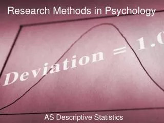
11. The Normal Distribution • in nature, the distribution of grouped frequencies of IQ, weight, height etc follow a normal (or Gaussian) distribution • symmetrical • bell-shaped • asymptotic • mean, median and mode coincide • income does not follow a normal distribution: power and resources are not distributed normally Research Methods in Politics CHapter 13

12. Questions for Discussion, Workshop Tasks or Assignments I • Access a UN, World Bank or EU data bank on the Internet, e.g., http://unstats.un.org/unsd/cdb/cdb or http://mdgs.un.org/unsd/unsd/ Choose a table of interest to you. Copy it to MS Excel. Calculate the summary descriptive statistics, 10th and 90th percentile. Compare the mean and median and explain the difference. 2. Create your own file of 1,000 random numbers using MS Excel. To do this click in turn on Tools in the menu bar then Random Number Generation. In the Random Number Generation Dialogue box, enter: Number of Variables (columns) = 10 Number of random numbers (rows) = 100 Distribution = normal Mean = 50 Standard deviation = 15 Random number seed = 5 Output Range = A1 Then click ‘OK’ Save as (file) Normal distribution random numbers. Then calculate the summary statistics for the entire data set. Retain the file for future use as your own bank of random numbers. Research Methods in Politics CHapter 13

13. Questions for Discussion, Workshop Tasks or Assignments II 3. Now analyse the random numbers above into a grouped frequency distribution. First, decide what class interval you wish to adopt. Your data extends from 0 to 100. You may decide to use a class interval of 5. Then enter 5 in cell K1 and continue to enter 10, 15, 20 etc until you reach 100 in cell K20. (You can, of course, use the Autofil routine). Then click on Tools and Data Analysis. In the Data Analysis dialogue box, click on Histogram and OK. In the Histogram dialogue box, insert ; Input Range A1:J100 Bin Range K1:K20 Output Range L1:L20 Then click on Chart Output and click OK. The output will appear: Now chart the distribution Research Methods in Politics CHapter 13

14. Questions for Discussion, Workshop Tasks or Assignments III Now chart the output You will note that the histogram apparently takes the shape of a uniform distribution. However, as we constructed our 1,000 cell bank of random numbers from a normal distribution, the chart is reassuring rather than surprising. But note how, despite having been calculated from 1,000 random numbers, the histogram does not follow a perfect uniform distribution: there will always be some variations from the perfect normal distribution when bins are used. Research Methods in Politics CHapter 13