6.4 Exponential Growth and Decay
120 likes | 358 Vues
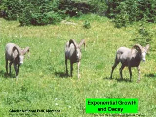
6.4 Exponential Growth and Decay. Glacier National Park, Montana Photo by Vickie Kelly, 2004. Greg Kelly, Hanford High School, Richland, Washington.

6.4 Exponential Growth and Decay
E N D
Presentation Transcript
6.4 Exponential Growth and Decay Glacier National Park, Montana Photo by Vickie Kelly, 2004 Greg Kelly, Hanford High School, Richland, Washington
The number of bighorn sheep in a population increases at a rate that is proportional to the number of sheep present (at least for awhile.) So does any population of living creatures. Other things that increase or decrease at a rate proportional to the amount present include radioactive material and money in an interest-bearing account. If the rate of change is proportional to the amount present, the change can be modeled by:
Rate of change is proportional to the amount present. Divide both sides by y. Integrate both sides.
Integrate both sides. Exponentiate both sides. When multiplying like bases, add exponents. So added exponents can be written as multiplication.
Since is a constant, let . Exponentiate both sides. When multiplying like bases, add exponents. So added exponents can be written as multiplication.
At , . Since is a constant, let . This is the solution to our original initial value problem.
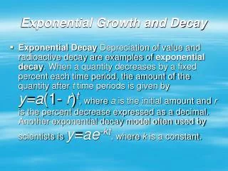
Note: This lecture will talk about exponential change formulas and where they come from. The problems in this section of the book mostly involve using those formulas. There are good examples in the book, which I will not repeat here. Exponential Change: If the constant k is positive then the equation represents growth. If k is negative then the equation represents decay.
Continuously Compounded Interest If money is invested in a fixed-interest account where the interest is added to the account k times per year, the amount present after t years is: If the money is added back more frequently, you will make a little more money. The best you can do is if the interest is added continuously.
You may also use: Continuously Compounded Interest: which is the same thing. Of course, the bank does not employ some clerk to continuously calculate your interest with an adding machine. We could calculate: but we won’t learn how to find this limit until chapter 8. (The TI-89 can do it now if you would like to try it.) Since the interest is proportional to the amount present, the equation becomes:
Radioactive Decay The equation for the amount of a radioactive element left after time t is: This allows the decay constant, k, to be positive. The half-life is the time required for half the material to decay.
Half-life: Half-life
Newton’s Law of Cooling where is the temperature of the surrounding medium, which is a constant. Newton’s Law of Cooling Espresso left in a cup will cool to the temperature of the surrounding air. The rate of cooling is proportional to the difference in temperature between the liquid and the air. (It is assumed that the air temperature is constant.) If we solve the differential equation: we get: p