Overview of Heuristic Search Strategies: AIMA 2nd Edition, Chapter 4.1-4.3
This document provides a comprehensive overview of heuristic search strategies as discussed in AIMA (Artificial Intelligence: A Modern Approach) 2nd Edition, specifically in Chapters 4.1 to 4.3. It covers fundamental concepts of blind tree search algorithms, including breadth-first search (BFS) and depth-first search (DFS), alongside informed searches such as best-first search, greedy search, and A* search. The text highlights the evaluation functions, properties, and optimality conditions of these search strategies along with their performance in various examples, including maze and Romanian map problems.

Overview of Heuristic Search Strategies: AIMA 2nd Edition, Chapter 4.1-4.3
E N D
Presentation Transcript
Heuristic search Reading: AIMA 2nd ed., Ch. 4.1-4.3 Rutgers CS440, Fall 2003
(Blind) Tree search so far • functionTreeSearch(problem, fringe) • n = InitialState(problem); • fringe = Insert(n); • while (1) • If Empty(fringe) return failure; • n = RemoveFront(fringe); • If Goal(problem,n) returnn; • fringe = Insert( Expand(problem,n) ); • end • end • Strategies: • BFS: fringe = FIFO • DFS: fringe = LIFO • Strategies defined by the order of node expansion Rutgers CS440, Fall 2003
Example of BFS and DFS in a maze G G s0 s0 Rutgers CS440, Fall 2003
Informed searches: best-first search • Idea: Add domain-specific information to select the best path to continue searching along. • How to do it? • Use evaluation function, f(n), which selects the most “desirable” (best-first) node to expand. • Fringe is a queue sorted in decreasing order of desirability. • Ideal case: f(n) = true cost to goal state = t(n) • Of course, t(n) is expensive to compute (BFS!) • Use an estimate (heuristic) instead Rutgers CS440, Fall 2003
maze example • f(n) = straight-line distance to goal 2 1 G 3 2 1 1 4 3 2 2 2 s0 3 3 3 4 4 4 Rutgers CS440, Fall 2003
Romania example Rutgers CS440, Fall 2003
Greedy search • Evaluation function f(n) = h(n) --- heuristic = estimate of cost from n to closest goal • Greedy search expands nodes that appear to be closest to goal Rutgers CS440, Fall 2003
Sibiu h = 253 Timisoara h = 329 Zerind h = 374 Arad h = 366 Fagaras h = 176 Oradea h = 380 Rimnicu V. h = 193 Sibiu h = 253 Bucharest h = 0 Example of greedy search Arad h = 366 Arad h = 366 Sibiu h = 253 Fagaras h = 176 Bucharest h = 0 Is this the optimal solution? Rutgers CS440, Fall 2003
Properties of greedy search • Completeness: • Not complete, can get stuck in loops, e.g., Iasi -> Neamt -> Iasi -> Neamt -> … • Can be made complete in finite spaces with repeated-state checking • Time complexity: • O(bm), but good heuristic can give excellent improvement • Space complexity: • O(bm), keeps all nodes in memory • Optimality: • No, can wander off to suboptimal goal states Rutgers CS440, Fall 2003
A-search • Improve greedy search by discouraging wandering-off • f(n) = g(n) + h(n)g(n) = cost of path to reach node nh(n) = estimated cost from node n to goal nodef(n) = estimated total cost through node n • Search along most promising path, not node • Is A-search optimal? Rutgers CS440, Fall 2003
Optimality of A-search • Theorem: Let h(n) be at most higher than t(n), for all n. Than, the A-search will be at most “steps” longer than the optimal search. • Proof: If n is a node on the path found by A-search, then f(n) = g(n) + h(n) g(n) + t(n) + = optimal + Rutgers CS440, Fall 2003
A* search • How to make A-search optimal? • Make = 0. • This means heuristic must always underestimate the true cost to goal. h(n) has to be an Optimistic estimate. • 0 h(n) t(n) is called an admissible heuristic. • Theorem: Tree A*-search is optimal if h(n) is admissible. Rutgers CS440, Fall 2003
Sibiu 393 = 140+253 Timisoara 477 = 118+329 Zerind 449 = 75+374 Arad 646 = 280+366 Fagaras 415 = 239+176 Oradea 671 = 291+380 Rimnicu V. 413 = 220+193 Craiova 526 = 366+160 Pitesti 417 = 317+100 Sibiu 553 = 300+253 Sibiu 591 = 338+253 Bucharest 450 = 450+0 Bucharest f = 418+0 Craiova 615 = 455+160 Rimnicu V. 607 = 414+193 Example of A* search Arad Arad h = 366 Sibiu Fagaras Rimnicu V. Pitesti Bucharest f = 418+0 Rutgers CS440, Fall 2003
s n G’ G A* optimality proof • Suppose there is a suboptimal goal G’ on the queue. Let n be an unexpanded node on a shortest path to optimal goal G. • f(G’) = g(G’) + h(G’) = g(G’) since h(G’)=0> g(G) since G’ is suboptimal f(n) = g(n) + h(n) since h is admissible • Hence, f(G’) > f(n), and f(G’) will never be expanded • Remember example on the previous page? Rutgers CS440, Fall 2003
Consistency of A* • Consistency condition:h(n) - c(n,n’) h(n’) where n’ is any successor of n • Guarantees optimality of graph search (remember, the proof was for tree search!) • Also called monotonicity:f(n’) = g(n’) + h(n’) = g(n) + c(n,n’) + h(n’) g(n) + h(n) = f(n)f(n’) f(n) • f(n) is monotonically non-decreasing Rutgers CS440, Fall 2003
Example of consistency/monotonicity • A* expands nodes in order of increasing f-value • Adds “f-contours” of nodes • BFS adds layers Rutgers CS440, Fall 2003
Properties of A* • Completeness: • Yes (for finite graphs) • Time complexity: • Exponential in | h(n) - t(n) | x length of solution • Memory requirements: • Keeps all nodes in memory • Optimal: • Yes Rutgers CS440, Fall 2003
Admissible heuristics h(n) • Straight-line distance for the maze and Romanian examples • 8-puzzle: • h1(n) = number of misplaced tiles • h2(n) = number of squares from desired location of each tile (Manhattan distance) • h1(S) = 7 • h2(S) = 4+0+3+3+1+0+2+1 = 14 Rutgers CS440, Fall 2003
Dominance • If h1(n) and h2(n) are both admissible and h1(n) h2(n), then h2(n) dominates over h1(n) • Which one is better for search? • h2(n), because it is “closer” to t(n) • Typical search costsd = 14, IDS = 3,473,941 nodes A*(h1) = 539 A*(h2) = 113d = 24, IDS ~ 54 billion nodes A*(h1) = 39135 A*(h2) = 1641 Rutgers CS440, Fall 2003
Relaxed problems • How to derive admissible heuristics? • Can be derived from exact solutions to problems that are “simpler” (relaxed) versions of the problem one is trying to solve • Examples: • 8-puzzle: • Tile can move anywhere from initial position (h1) • Tiles can occupy same square but have to move one square at a time (h2) • maze: • Can move any distance and over any obstacles • Important:The cost of optimal solution to relaxed problems is no greater than the optimal solution to the real problem. Rutgers CS440, Fall 2003
Local search • In many problems one does not care about the path, rather one wants to find the goal state (based on a goal condition). • Use local search / iterative improvement algorithms: • Keep a single “current” state, try to improve it. Rutgers CS440, Fall 2003
Example • N-queens problem:from initial configuration move to other configurations such that the number of conflicts is reduced Rutgers CS440, Fall 2003
Hill-climbingGradient ascent / descent • Goal:n* = arg max Value( n ) • functionHillClimbing(problem) • n = InitialState(problem); • while (1) • neighbors = Expand(problem,n); • n* = arg max Value(neighbors); • If Value(n*) < Value(n), return n; • n = n*; • end • end Rutgers CS440, Fall 2003
Hill climbing (cont’d) • Problem:Depending on initial state, can get stuck in local maxima (minima), ridges, plateaus Rutgers CS440, Fall 2003
Beam search • Problem of local minima (maxima) in hill-climbing can be alleviated by starting HC from multiple random starting points • Or make it stochastic (Stochastic HC) by choosing successors at random, based on how “good” they are • Local beam search: somewhat similar to random-restart HC: • Start from N initial states. • Expand all N states and keep N best successors. • Stochastic beam search: stochastic version of LBS, similar to SHC. Rutgers CS440, Fall 2003
Simulated annealing • Idea: • Allow bad moves, initially more, later fewer • Analogy with annealing in metallurgy • functionSimulatedAnnealing(problem,schedule) • n = InitialState(problem); • t = 1; • while (1) • T = schedule(t); • neighbors = Expand(problem,n); • n’ = Random(neighbors); • V = Value(n’) - Value(n); • IfV > 0, n* = n; • Elsen* = n’ with probability exp(V/T); • t = t + 1; • end • end Rutgers CS440, Fall 2003
Properties of simulated annealing • At fixed temperature T, state occupation probability reaches Boltzman distribution, exp( V(n)/T ) • Devised by Metropolis et al. in 1953 Rutgers CS440, Fall 2003
Genetic algorithms Rutgers CS440, Fall 2003