Reachability, Schedulability and Optimality
Reachability, Schedulability and Optimality. Ansgar Fehnker. June 3. Outline. Timed automata a la Uppaal From Reachability to Schedulability LPTAs Priced regions and operations Algorithm Termination Priced Zones Verification vs. Optimization Guiding and Bounding examples

Reachability, Schedulability and Optimality
E N D
Presentation Transcript
Reachability, Schedulability and Optimality Ansgar Fehnker June 3
Outline • Timed automata a la Uppaal • From Reachability to Schedulability • LPTAs • Priced regions and operations • Algorithm • Termination • Priced Zones • Verification vs. Optimization • Guiding and Bounding • examples • examples
Timed Automata (UPPAAL) • Network of Automata • Synchronization (CCS-like) a! a?
Timed Automata (UPPAAL) • Network of Automata • Synchronization (CCS-like) • Clocks in description • Time passes uniformly • Guard/reset on action • Invariants on location x 7 3 x 7 y > 4 a! a? y:=0 Uppaal is a modelchecker forTimed Automata with emphasis on reachability properties
25min 20min 10min 5min Can they make it within 60 minutes ? Unsafe Safe Motivation Observation Many scheduling problems can be phrased in a natural way as reachability problems for timed automata!
unsafe unsafe unsafe take? take? L==0 L==0 L==0 unsafe take! y:=0 take! y:=0 take! y:=0 y>=20 y>=10 y>=5 release? release? L==0 release! release! release! release! release! release! L:=1-L L==1 L==1 L==1 y>=25 take! y:=0 y>=25 y>=25 y>=25 take! y:=0 take! y:=0 take! y:=0 safe safe safe release! release! L==1 y>=25 take! y:=0 safe Motivation 25min 20min 10min 5min What schedule minimizes crossings? What is the fastest schedule? Can they make it within 60 minutes ? What schedule mini-mizes unsafe time? Unsafe Safe
cost’=1 cost’=2 cost’=0 x<5 x<3 cost+=4 y>2 c a b y:=0 (2.5) (a,x=y=0) (b,x=y=0) (b,x=y=2) (a,x=0,y=2) 4 2.5 x 2 0 Linearly Priced Timed Automata • Timed Automata + Costs on transitions and locations. • Cost of performing transition: Transition cost. • Cost of performing delay d: ( d x location cost ). • Cost of Execution Trace: Sum of costs: 4 + 5 + 0 = 9
cost E earliest landing time T target time L latest time ecost rate for being early l cost rate for being late dfixed cost for being late d+l*(t-T) e*(T-t) t E T L Example: Aircraft Landing Planes have to keep separation distance to avoid turbulences caused by preceding planes Runway
Example: Aircraft Landing x <= 5 x=5 x >= 4 4 earliest landing time 5 target time 9 latest time 3cost rate for being early 1 cost rate for being late 2fixed cost for being late land! cost+=2 x <= 5 x <= 9 cost’=3 cost’=1 x=5 land! Planes have to keep separation distance to avoid turbulences caused by preceding planes Runway
delay 1 y 0 x -2 x-y 0 Zones Basic idea: Define a delay and reset over zones 1 y 4 0 x 3 -2 x-y 0 y x x<3 x<3 y>2 c a b y:=0
reset y 0 y 0 0 x 3 Zones Basic idea: Define a delay and reset over zones 1 y 4 0 x 3 -2 x-y 0 y x x<3 x<3 y>2 c a b y:=0
cost’=1 cost’=2 cost’=0 cost+=4 3 -1 0 delay 2 cost=c’’ -1 x + 3 y cost=c’+ 0 x + 2 y cost=c - 1 x + 2 y Priced Zones Basic idea: Define a linear cost function on zones cost = c - 1 x + 2 y y 2 -1 x x<5 x<3 y>2 c a b y:=0
reset y cost = c - 1 x cost = c’+ 1 x -1 1 Priced Zones Basic idea: Define a delay and reset over zones cost = c - 1 x + 2 y y 2 -1 x x<3 x<3 y>2 c a b y:=0
Cost=60 An Algorithm • State-Space Exploration + Use of global variable Cost. • Updated Cost whenever goal state with min( C ) <Cost is found: Cost= Cost=80 80 60
An Algorithm Cost:=, Pass := {}, Wait := {(l0,C0)}, Goal= while Wait {} do select (l,C) from Wait if (l,C)= and mincost(C)<Cost then Cost:=mincost(C) if forall (l’,C’) in Pass: C’ C then add (l,C) to Pass forall (m,D) such that (l,C) (m,D): add (m,D) to Wait Return Cost
An Algorithm Cost:=, Pass := {}, Wait := {(l0,C0)}, Goal= while Wait {} do select (l,C) from Wait if (l,C)= and mincost(C)<Cost then Cost:=mincost(C) if forall (l’,C’) in Pass: C’ C then add (l,C) to Pass forall (m,D) such that (l,C) (m,D): add (m,D) to Wait Return Cost Performs: symbolic operations Delay, Conjun-ction, and Reset of clocks.
C C’ C’ isbigger & cheaper than C is a well-quasi ordering which guarantees termination! An Algorithm Cost:=, Pass := {}, Wait := {(l0,C0)}, Goal= while Wait {} do select (l,C) from Wait if (l,C)= and mincost(C)<Cost then Cost:=mincost(C) if forall (l’,C’) in Pass: C’ C then add (l,C) to Pass forall (m,D) such that (l,C) (m,D): add (m,D) to Wait Return Cost .
Theorem When the algorithm terminates, the value of COSTequals mincost(). An Algorithm Cost:=, Pass := {}, Wait := {(l0,C0)}, Goal= while Wait {} do select (l,C) from Wait if (l,C)= and mincost(C)<Cost then Cost:=mincost(C) if forall (l’,C’) in Pass: C’ C then add (l,C) to Pass forall (m,D) such that (l,C) (m,D): add (m,D) to Wait Return Cost
Verification vs. Optimization Safe side reachable? • Verification Algorithms: • Checks a logical property for the entire state-space • Efficient blind search. • Optimization Algorithms: • Finds (near) optimal solutions. • Uses techniques to avoid non-optimal parts of the state-space (e.g. Branch and Bound). • Objective: • Bridge the gap between these two. • New techniques and applications in UPPAAL. 80 Min time of reaching safe side? 60
Minimum-Cost Order • The basic algorithm finds the minimum cost trace. • Breadth or Depth-first search-order. • Problem: Searches the entire state-space. • Minimum-Cost Search Order: Always explore state with smallest minimum cost first.
Minimum-Cost Order Fact: First found goal state is optimal. • Cost grows along all paths. • The search can terminate when first goal state found. • Like Dijkstra’s shortest path algorithm. • Simpler algorithm: variable Cost no longer needed.
Estimates of Remaining Cost • Often a conservative estimate of the remaining cost can be found. • REM( l, C ) = conservative estimate of remaining cost. • Bridge example: REM( l, C ) = time of slowest person on Unsafe side. At least 25 mins needed to complete schedule.
Estimates of Remaining Cost • Basic Algorithm + Estimate of remaining cost:Only states with (min(C) + REM(l, C)) < Cost are further explored. Cost=80 min( C ) + REM( l, C ) 80
Estimates of Remaining Cost • Basic Algorithm + Estimate of remaining cost:Only states with (min(C) + REM(l, C)) < Cost are further explored. • Minimum Cost + Estimate of remaining cost:Explore states with smallest ( min(C) + REM( l, C ) ) first. Cost=80 min( C ) + REM( l, C ) 80
Using Heuristics • Allows the users to control the search order according to heuristics. • Symbolic states extended to (l, C, h), whereh is the priority of a state. • Transitions are annotated with assignments to h. • Flexible! Basic Algorithm + Heuristics:State with highest h is explored first.
Using Heuristics Try to schedule planes in the order of their preferred landing times
Aircraft Landing Problem runways Benchmark by Beasley et al 2000
Example: Bridge Problem What is the fastest schedule? • Number of symbolic states generated with cost-extended version of UPPAAL. • Minimum Cost Order + Estimate of Remaining cost<10% of Breadth-First Search. BF = Breadth-First, DF = Depth-First, MC = Minimum Cost Order, MC+ = MC + REM
SIDMAR Steel Production Plant Crane A Machine 2 Machine 3 Machine 1 • A. Fehnker [RTCSA99], T. Hune, K. G. Larsen, P. Pettersson [DSV00] • Case study of Esprit-LTRproject 26270 VHS • Physical plant of SIDMARlocated in Gent, Belgium. • Part between blast furnace and hot rolling mill. Objective:model the plant, obtain schedule and control program for plant. Lane 1 Machine 4 Machine 5 Lane 2 Buffer Crane B Storage Place Continuos Casting Machine
SIDMAR Steel Production Plant Crane A Input: sequence of steel loads (“pigs”). Machine 2 Machine 3 Machine 1 @10 @20 2 @10 2 2 Lane 1 Machine 4 Machine 5 15 @10 Load follows Recipe to obtain certain quality, e.g: start; T1@10; T2@20; T3@10; T2@10; end within 120. Lane 2 16 Buffer Crane B =127 Storage Place Good schedules forten batcheswithin seconds, rather than bad schedules for five batches within almost an hour. @40 Continuos Casting Machine Output: sequence of higher quality steel.
SIDMAR Steel Production Plant crane a • LEGO RCX Mindstorms. • Local controllers with control programs. • IR protocol for remote invocation of programs. • Central controller. m1 m2 m3 m4 m5 crane b buffer storage central controller casting Synthesis
Heuristics: BPM protocol Heuristic: search first for constant input 1 Up to 50% reduction for erroneous instances of a simple communcation protocol.
Conclusion • Advantages • Easy and flexible modeling of systems • Whole range of verification techniques becomes available • Controller/Program synthesis • Disadvantages • Existing scheduling approaches perform somewhat better • Our goal • See how far we get; • Integrate model checking and scheduling theory. • Future work • Tailoring Linear Programming to Priced Zones • Translation trace to schedule, re-use of schedules, ...
Related Work • Alur, Courcourbetis, Henzinger (1993)Accumulated delays in Realtime Systems • Alur, Torre, Pappas (HSCC’01)Optimal Paths in Weighted Timed Automata • Behrmann, Fehnker, et all (HSCC’01)Minimum-Cost Reachability for Priced Timed Automata
Related Work (cont) • Asarin & Maler (1999)Time optimal control using backwards fixed point computation • Niebert, Tripakis & Yovine (2000)Minimum-time reachability using forward reachability • Behrmann, Fehnker et all (TACAS’2001, CAV’01)Minimum-time reachability using Branch-and-Bound • Brinksma, Maler, Fehnker(STTT02) Using UPPAAL en SPIN to compute optimal schedules. • Abdeddaim, Maler (CAV’01)Job-Shop Scheduling using Timed Automata • General Trend (AAAI’01):Integrating Scheduling/Planning and Model Checking
cost’=1 cost’=2 cost’=0 x<3 x<3 cost+=4 y>2 c a {x:=0} (2.5) (a,x=y=0) (b,x=y=0) (b,x=y=2) (a,x=0,y=2) 4 2.5 x 2 0 Linearly Priced Timed Automata • Timed Automata + Costs on transitions and locations. • Cost of performing transition: Transition cost. • Cost of performing delay d: ( d x location cost ). b • Cost of Execution Trace: Sum of costs: 4 + 5 + 0 = 9
y 5 4 3 2 1 x 0 1 2 3 4 5 Regions x<3 x<3 y>2 c a b {x:=0}
y 5 4 3 2 1 x 0 1 2 3 4 5 Regions x<3 x<3 y>2 c a b {x:=0}
3 3 3 2 2 2 1 1 1 x x x Alur & Dill Regions x<3 x<3 y>2 c a b {x:=0} y y y 1 2 3 1 2 3 1 2 3 Transitions with and w/o reset and delay can be considered as transitions on regions!