
Use of Matrix P opulation M odels in Ecology and Conservation Biology II
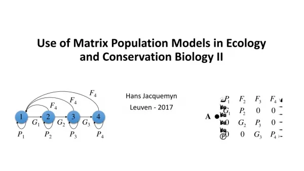
Use of Matrix P opulation M odels in Ecology and Conservation Biology II. F 4. Hans Jacquemyn Leuven - 2017. F 4. F 4. 1. 2. 3. 4. G 1. G 2. G 3. P 1. P 2. P 3. P 4. 6. Perturbation analysis. 6.1 Introduction

Use of Matrix P opulation M odels in Ecology and Conservation Biology II
E N D
Presentation Transcript
Use of Matrix Population Models in Ecology and Conservation Biology II F4 Hans Jacquemyn Leuven - 2017 F4 F4 1 2 3 4 G1 G2 G3 P1 P2 P3 P4
6. Perturbation analysis • 6.1 Introduction • The results of a matrix population analysis is a set of demographic statistics (population growth rate, stable stage distribution, reproductive value, ...). • Those statistics are functions of the vital rates, and through them of biological and environmental variables. • However, the vital rates might have been otherwise, and had they been, the results of the analysis would have been different. • Perturbation analysis asks what would happen if one or more independent variables were to change. • Prospective and retrospective perturbation analysis
6. Perturbation analysis • 6.2 Sensitivity analysis • The sensitivity (sij) is the local slope of λ, considered as a function of aij: • Population growth rate is most sensitive to changes in the vital rates displaying the largest sensitivities • The sensitivities of λ to all of the aij are calculated and displayed in a sensitivity matrixS. where wj is the jth element of the right eigenvector w, vi is the ith element of the left eigenvector v, and <w,v> denotes the scalar product.
6. Perturbation analysis • 6.2 Sensitivity analysis
6. Perturbation analysis • 6.2 Sensitivity analysis λ = 1.060 λ’ = 0.827 / 22.0% reduction λ’’ = 1.032, 2.7% reduction
6. Perturbation analysis 6.2 Sensitivity analysis
6. Perturbation analysis 6.2 Sensitivity analysis stages <- c("seedling", "juvenile", "non-flow", "flowering"); A <- matrix(c(0,0,0,0.10,0.98,0.32,0,0,0,0.61,0.51,0.10,0,0.08,0.47,0.90), byrow=TRUE, ncol=4, dimnames=list(stages,stages)); A; seedling juvenile non-flow flowering seedling 0.00 0.00 0.00 0.1 juvenile 0.98 0.32 0.00 0.0 non-flow 0.00 0.61 0.51 0.1 flowering 0.00 0.08 0.47 0.9 sens <- sensitivity(A, zero=TRUE); sens; seedling juvenile non-flow flowering seedling 0.00000000 0.00000000 0.0000000 0.5189535 juvenile 0.05295444 0.07009116 0.0000000 0.0000000 non-flow 0.00000000 0.07374801 0.1890790 0.5908242 flowering 0.00000000 0.08636330 0.2214228 0.6918903
6. Perturbation analysis 6.2 Sensitivity analysis image2(sens, mar=c(1,5,5,1), box.offset=.1);
6. Perturbation analysis • 6.3 Elasticity analysis • Transition probabilities, which can not exceed 1, and fertilities, which are under no such restriction, are measured on different scales. • This has led many researchers to consider the response to a proportional, rather than absolute, perturbations. • The proportional response to a proportional perturbation is known as elasticity in economics. • In matrix models, the elasticity eij of λ with respect to aijis defined as: • The elasticity eijis the slope of log λ plotted against log aij. Since equal increments on a log scale correspond to equal proportions on an arithmetic scale, elasticity measures proportional sensitivity.
6. Perturbation analysis 6.3 Elasticity analysis elas <- elasticity(A); elas; seedling juvenile non-flow flowering seedling 0.00000000 0.000000000 0.00000000 0.04893951 juvenile 0.04893951 0.021151655 0.00000000 0.00000000 non-flow 0.00000000 0.042423966 0.09093785 0.05571722 flowering 0.00000000 0.006515539 0.09814119 0.58723357 image2(elas, mar=c(1,5,5,1), box.offset=.1)
6. Perturbation analysis 6.3 Elasticity analysis
6. Perturbation analysis • 6.4 Sensitivity vs. elasticity analysis • Sensitivity sij quantifies the absolute change in λ of an infinitesimalabsolute change in matrix transition aij. • Elasticityeij quantifies the proportional change in λresultingfrom an infinitesimalproportional change in matrix transition aij. • An important characteristicisthat all elasticities of a transition matrix sum to one: • Comparison of the relative importance of different types of transitions
6. Perturbation analysis • 6.5 Comparative analysis of elasticity values • The fact that elasticities sum to one allows making comparisons among populations and species. • One approach sums the elasticities of different kinds of transitions: stasis, growth and fertility. Survival elasticity: S22 + S33 + S34 + S44 Growth elasticity: G21 + G32 + G43 Fecundity elasticity: F14
6. Perturbation analysis 6.5 Comparative analysis of elasticity values
6. Perturbation analysis 6.5 Comparative analysis of elasticity values Grassland Heathland F : 0.063 0.195 L: 0.702 0.412 G : 0.235 0.393 Heathland Grassland
6. Perturbation analysis 6.5 Comparative analysis of elasticity values Oostermeijeret al. (1996) Journal of Ecology 84: 153-166
6. Perturbation analysis 6.5 Comparative analysis of elasticity values Franco & Silvertown (1996) Phil Trans Roy Soc London B 351: 1341-1348
VITAL RATES POPULATION STATISTICS E1 P1 A(1) . . . . . . . . VITAL RATES POPULATION STATISTICS PN EN A(N) 6. Perturbation analysis • 6.6 Life Table Response Experiments • Populations occur in different environments. These different environments may largely affect the vital rates, and thus population demography. • The effects on the vital rates are usually diverse and mostly stage-specific. • Demographic models provide a tool to synthesize these effects into statistics that quantify the effects of different environments at the level of the population.
6. Perturbation analysis • 6.6 Life Table Response Experiments • Decomposition of the effects of population (or treatment) on λ into contributions arising from the effect of each stage-specific vital rates allows answering questions such as: • Are low growth rates in one population the effect of increased mortality, decreased fecundity or a combination? • Are these effects all equally responsible for the effect on λ, or can parts of that effect be attributed to each of them? • To answer these questions requires a decomposition of the effect of population (or treatment) on λ into contributions arising from the effect on each stage-specific vital rate. • There are several decomposition techniques, but here we focus only on fixed one-way designs.
6. Perturbation analysis • 6.6 Life Table Response Experiments • Consider a one-way design with two treatments T1 and T2 producing population growth rates λ(1) and λ(2). • Choose a reference matrix A(r) as a baseline against which to measure treatment effects. A(r) might be the mean matrix A(•) or the matrix for a particular level of the treatment, often the control. • Expanding λ, as a function of the aij, around A(r) gives the population growth rate in treatment m as: • where . • The terms in the summation term are the contributions of the aijto the effect of treatmentm on population growth.
6. Perturbation analysis 6.6 Life Table Response Experiments Example: Gentiana pneumonanthe λ(2) = 0.934 λ(1) = 1.151
6. Perturbation analysis 6.6 Life Table Response Experiments Example: Gentiana pneumonanthe
6. Perturbation analysis 6.6 Life Table Response Experiments Example: Gentiana pneumonanthe Contributions to differences in λ:
6. Perturbation analysis 6.6 Life Table Response Experiments Calculation in R stages <- matrix(c("seedling","juvenile","vegetative","flowering","dormant"), byrow=TRUE, ncol=1); heathland <- matrix(c(0,0,0,3.179,0,0.047,0.001,0,2.065,0,0.145,0.765,0.538,0.289,0.333,0.007,0.048,0.131,0.502,0.167,0.010,0.009,0.048,0.030,0.500), byrow=TRUE, ncol=5, dimnames=list(stages,stages)); heathland; lambda(heathland); grassland <- matrix(c(0,0,0,0.442,0,0.027,0,0,0.164,0,0.170,0.675,0.533,0.251,0.579,0,0.013,0.172,0.658,0.159,0.002,0.049,0.039,0.040,0.262), byrow=TRUE, ncol=5, dimnames=list(stages,stages)); grassland; lambda(grassland);
6. Perturbation analysis 6.6 Life Table Response Experiments Calculation in R Cm <- LTRE(heathland, grassland); seedling juvenile vegetative flowering dormant seedling 0.000000000 0.0000000000 0.000000000 0.070707176 0.000000000 juvenile 0.003616307 0.0001175902 0.000000000 0.203879771 0.000000000 vegetative -0.005663574 0.0132595552 0.001813033 0.005106119 -0.009269456 flowering 0.004998118 0.0162522096 -0.046857315 -0.066067798 0.000950095 dormant 0.002536528 -0.0082479419 0.004567487 -0.001880643 0.012551489
6. Perturbation analysis 6.6 Life Table Response Experiments Example: Gentiana pneumonanthe FsfFjfajsavsafsavs adsajjavjafjadjavvafvadvavfaffadfavdafd add Life cycle transition
6. Perturbation analysis • 6.6 Life Table Response Experiments • Difference between prospective and retrospective perturbation analysis • Prospective analysis (sensitivity and elasticity analysis) explores the functional dependence of λ on the vital rates. Prospective analysis looks forward and asks what will happen if aij is perturbed. It cannot reveal anything about how the vital rates varied in the past, are varying now, or might vary in the future. • Retrospective analysis (LTRE) looks at variation in vital rates, and how this variation contributes to variation in λ. Retrospective analyses can therefore diagnose causes of observed changes in λ, but cannot predict the effects of future management, because future management actions bear no necessary relation to past changes.
7. Stochastic matrix models • 7.1 Introduction • Up till now, we have considered models in which the environment does not change in time. This is usually not the case, and often the environment, and thus the vital rates, vary randomly over time. This is called environmental stochasticity. • A stochastic matrix model contains three parts: • A stochastic model that produces a sequence of environmental states • A function that associates a matrix with each environmental state • A sequence of population vectors n(t) that results from applying the series of matrices to an initial population vector n(0). • The population growth rate for stochastic environments is called the stochastic population growth rate. • Temporal variability should generally decrease the long- term population growth rate.
7. Stochastic matrix models 7.2 Calculation of the stochastic growth rate - simulation Consider a stochastic sequence of matrices A0, A1, ..., At-1 and an initial population vector n(0)= n0 The population size at time t is N(t) = ǁn(t)ǁ = ǁAt-1At-2...A0n0ǁ It can then be proven there exists a number λssuch that The quantity log λs is called the stochastic growth rate. It is a fixed, nonrandom quantity that is independent of n0.
7. Stochastic matrix models 7.2 Calculation of the stochastic growth rate - simulation The stochastic growth rate can be estimated from the average growth rate over a long simulation as: It is equivalent to calculating the amount by which the population grows at each time step and then averaging the results: The precision of this estimate can be measured by calculating the variance V of each of the proportions of log (N(t+1)/N(t)).
7. Stochastic matrix models 7.3 Calculation of the stochastic growth rate – Lewontin-Cohen model Consider that population size N grows from time t to t + 1 as a factor of the temporally varying geometric population growth rate λt, such that Nt+1 = Ntλt. If λt is a random variable with expected value (arithmetic mean) E[λt] and variance Var(λt), the long- term stochastic population growth rate λs is approximated by: Thus, an increase in variability is expected to decrease long-term population growth, all else equal.
7. Stochastic matrix models • 7.4 Example: Polar bear (Ursus maritimus) • Climate change is predicted to have significant effects on population dynamics, species distributions and interactions, food web structure and biodiversity. • The climate is changing faster in the Arctic than anywhere else. • For Arctic marine mammals, the most critical of these changes involve the sea ice environment. • The Polar bear (Ursusmaritimus) is one of the most ice-dependent of all Arctic marine mammals
7. Stochastic matrix models 7.4 Example: Polar bear (Ursusmaritimus) 3 1 2 4 6 5 1 – 3: non-reproductive females aged 2, 3 and 4 years, respectively; 4: adult females available to breed; 5: females accompanied with cubs of the year; 6: females accompanied by one or more yearling cubs Hunter et al. (2010) Ecology 91: 2883-2897
7. Stochastic matrix models 7.4 Example: Polar bear (Ursusmaritimus) Hunter et al. (2010) Ecology 91: 2883-2897
7. Stochastic matrix models 7.4 Example: Polar bear (Ursus maritimus) Population growth rate Number of ice-free days Hunter et al. (2010) Ecology 91: 2883-2897
7. Stochastic matrix models 7.4 Example: Polar bear (Ursus maritimus) Life Table Response Experiment (LTRE)
7. Stochastic matrix models 7.4 Example: Polar bear (Ursus maritimus) polarbear <- list(a2001,a2002,a2003,a2004,a2005); polarbear; sgr <- stoch.growth.rate(polarbear); sgr; $approx [1] -0.07417342 $sim [1] -0.07319044 $sim.CI [1] -0.07443117 -0.07194971 exp(sgr$approx); [1] 0.9635547
7. Stochastic matrix models 7.4 Example: Polar bear (Ursus maritimus)
7. Stochastic matrix models 7.4 Example: Polar bear (Ursus maritimus) Stochastic simulations with q the probability of a poor ice year. x.eq <- stoch.projection(polarbear, n, nreps = 1000); x.uneq <- stoch.projection(polarbear, n, nreps = 1000, prob = c(.2,.2,.2,.1,.1)); Hunter et al. (2010) Ecology 91: 2883-2897
Overview • Part I: Theory and Models • Introduction • Age-classified matrix models • Stage-classified matrix models • The matrix model • Statistical Inference • Perturbation analysis • Stochastic matrix models • Part II: Applications • Glossary • Conservation Biology • Assessment • Diagnosis • Prescription • Prognosis • Pest control • Reducing pest population size • Slowing or halting the invasion of the pest population
2. Conservation Biology • 2.1 Introduction • Demographic models are essential tools in conservation and population management since most management problems involve the vital rates. • Demographic models allow to address the following questions: • What is the status of the population? • Why is the status as it is? • What should be done about it? • What will happen if we do it?
2. Conservation Biology • 2.2 Matrix population models in conservation biology • 2.2.1 Assessment • What is the status of the population? Is it healthy or should we be worried about it and considering intervention? • Population growth rate plays the most central role in assessment. Negative growth rates will almost always result in extinction unless something changes them. • Because status assessment is an estimation problem, methods for quantifying the uncertainty in estimated parameters play a particularly important role.
2. Conservation Biology • 2.2 Matrix population models in conservation biology • 2.2.2 Diagnosis • The next step is to diagnose the causes of decline. • Diagnosis is inherently comparative. It seeks to answer why a population is in trouble and others are not, or why it is in trouble now but wasn’t before. • Diagnoses are therefore always phrased in terms of differences. • The primary tool is retrospective perturbation analysis (LTRE analysis).
2. Conservation Biology • 2.2 Matrix population models in conservation biology • 2.2.2 Diagnosis • Ideally, data from before and after the decline, should be available to quantify the contribution of vital rates to the changes in λ. • Unfortunately, such data are not available in most cases and other techniques have to be used to diagnose causes of decline. • However, if they were available, they certainly would have suggested further experiments to determine the environmental factors causing the changes in the vital rates.
2. Conservation Biology • 2.2 Matrix population models in conservation biology • 2.2.3 Prescription • Management strategies aim to improve population performance. They attempt to change the vital rates so that population growth rate λ increases. • In other words, management is perturbation, and the best tool for evaluating management prescriptions is prospective perturbation analysis, because it identifies the points in the life cycle where perturbations will have the largest effect on population growth. • These make attractive targets for management intervention.
2. Conservation Biology • 2.2 Matrix population models in conservation biology • 2.2.4 Prognosis • The goal of prognosis is to predict the population’s fate. • Population prognoses are also called population viability analyses (PVA). • The results of a PVA are often expressed as probabilities of extinction, or of population growth or decline over some specified time horizon. • Rather than describing current conditions (assessment), estimating the effects of past differences (diagnosis) or comparing the effects of hypothetical future changes (prescription), PVA attempts to say something about the future fate of the population.
2. Conservation Biology • 2.2 Matrix population models in conservation biology • 2.2.4 Prognosis • Population viability analysis is more difficult and risky than assessment, diagnosis or prescription. • A recent review pointed out most models failed to forecast the future of the populations that were studied. Predicted population size Observed population size 95% confidence interval
2. Conservation Biology 2.2 Matrix population models in conservation biology
2. Conservation Biology • 2.3 Examples • Example 1: Northern Atlantic whale (Eubalaenaglacialis) • Formerly abundant in the north-western Atlantic. • By 1900 almost hunted to extinction. • After the end of commercial whaling prospects were relatively good, with the population increasing again. • However, recent evidence indicates that it has been declining since about 1990. • At present there are only 300 individuals left and the species may already be functionally extinct owing to demographic stochasticity or the difficulty of females locating mates in the vast Atlantic Ocean.