Processing: zero-offset gathers
Processing: zero-offset gathers. The simplest data collection imaginable is one in which data is recorded by a receiver, whose location is the same as that of the source. This form of data collection is referred to as zero-offset gathers . Advantage: Easy to interpret.

Processing: zero-offset gathers
E N D
Presentation Transcript
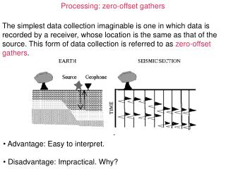
Processing: zero-offset gathers The simplest data collection imaginable is one in which data is recorded by a receiver, whose location is the same as that of the source. This form of data collection is referred to as zero-offset gathers. • Advantage: Easy to interpret. • Disadvantage: Impractical. Why?
Processing: common shot gathers Data collection in the form of zero-offset gathers is impractical, since very little energy is reflected by normal incidence. Thus, the signal-to-noise ratio is small. Seismic data is always collected in common shot gathers, i.e. multiple receivers are recording the signal originating from a single shot.
Processing: common midpoint gathers Common midpoint gathers: Regrouping the data from multiple sources such that the mid-points between the sources and the receivers are the same.
Processing: common depth gather For a horizontal flat layer on top of a half-space, the common mid-point gather is actually a common depth gather. In that case, the half offset between the shot and the receiver is located right above the reflector. (Next you will see that this is a very logical way of organizing the data.)
Processing: normal moveout correction Step 1: The data is organized into common mid-point gathers at each mid-point location. Step 2: Coherent arrivals are identified, and a search for best fitting depth and velocity is carried out.
Processing: normal moveout correction Step 3: The arrivals are aligned in a process called normal moveout correction (NMO), and the aligned records are stacked. If the NMO is done correctly, i.e. the velocity and depth are chosen correctly, the stacking operation results in a large increase of the coherent signal-to-noise ratio.
Processing: plotting the seismic profile The next step is to plot all the common mid-point stacked traces at the mid-point position. This results in a zero-offset stacked seismic section. At this stage, the vertical axis of the profile is in units of time (and not depth).
Processing The above section may be viewed as an ensemble of experiments performed using a moving zero-offset source-receiver pair at each position along the section. In summary, in reflection seismology, the incidence angle is close to vertical. This results in a weak reflectivity and small signal-to-noise ratio. To overcome this problem we perform normal moveout corrections followed by trace stacking. This results in a zerro-offset stack.
Processing: additional steps • Additional steps are involved in the processing of reflection data. The main steps are: • Editing and muting • Gain recovery • Static correction • Deconvolution of source • The order in which these steps are applied is variable.
Processing • Editing and muting: • Remove dead traces. • Remove noisy traces. • Cut out pre-arrival nose and ground roll. • Gain recovery: “turn up the volume” to account for seismic attenuation. • Accounting for geometric spreading by multiplying the amplitude with the reciprocal of the geometric spreading factor. • Accounting for anelatic attenuation by multiplying the traces by expt, where is the attenuation constant.
Processing: static (or datum) correction Time-shift of traces in order to correct for surface topography and weathered layer. Corrections: where: Es is the source elevation Er is the receiver elevation Ed is the datum elevation V is the velocity above the datum
Processing: static (or datum) correction An example of seismic profile before (top) and after (bottom) the static correction.
Processing: deconvolution of the source source wavelet reflectivity series output series Seismograms are the result of a convolution between the source and the subsurface reflectivity series (and also the receiver). Mathematically, this is written as: where the operator denotes convolution. In order to remove the source effect, one needs to apply deconvolution: where the operator denotes deconvolution.
Processing: deconvolution of the source Seismic profiles before (top) and after (bottom) the deconvolution. Note that the deconvolved signal is spike-like.
Processing: 3D reflection The 3D reflection experiments came about with the advent of the fast computers in the mid-1980’s. In these experiments, geophones and sources are distributed over a 2D ground patch. For example, a 3D reflectivity cube of data sliced horizontally to reveal a meandering river channel at a depth of more than 16,000 feet.
Processing: inclined interface The reflection point is right below the receiver if the layer is horizontal. For an inclined layer, on the other hand, the reflection bounced from a point up-dip. Thus the travel-time curve will show a reduced dip.
Processing: curved interface A syncline with a center of curvature that is located below the surface results in three normal incidence reflections.
Processing: migration Reflection seismic record must be corrected for non-horizontal reflectors, such as dipping layers, synclines, and more. Migration is the name given to the process which attempts do deal with this problem, and to move the reflectors to their correct position. The process of migration is complex, and requires prior knowledge of the seismic velocity distribution.