Download
1 / 63
640 likes | 1k Vues
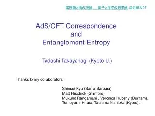
弦理論と場の理論 --- 量子と時空の最前線 @ 近畿大 07’. AdS/CFT Correspondence and Entanglement Entropy. Tadashi Takayanagi (Kyoto U.). Thanks to my collaborators: Shinsei Ryu (Santa Barbara)

E N D
弦理論と場の理論 --- 量子と時空の最前線@近畿大07’ AdS/CFT Correspondence andEntanglement Entropy Tadashi Takayanagi (Kyoto U.) Thanks to my collaborators: Shinsei Ryu (Santa Barbara) Matt Headrick (Stanford) Mukund Rangamani , Veronica Hubeny (Durham), Tomoyoshi Hirata, Tatsuma Nishioka (Kyoto) .
①Introduction Ten years have already been passed since the AdS/CFT correspondence was discovered by J. Maldacena. Many affirmative evidences have been accumulated for this conjectured duality, especially in the celebrated example of Therefore, nowadays, many people believe the AdS/CFT is true at least in this particular example.
UV-IR relation The coordinate z plays the role of length scale in the sense of the RG scale in QFT. The boundary z=0 corresponds to the UV limit.
Boundary 1/z ∝ The energy of extended F-string
Also many other successful examples have been found. (i) The deformation of (i.e. R-sym) This leads to less supersymmetric CFTs.
(ii) The deformation of (UV-IR relation) horizon AdSBH UV IR capped off AdS
In spite of these remarkable development, we still do not clearly understand the reason why the AdS/CFT is true. Remember that the AdS/CFT is an explicit realization of holography. A systematic proof of AdS/CFT will be related to the proof of the holography itself. The idea of holography Often, lives in the boundary of (d+2) dim. spacetime (d+2) dimensional (d+1) dimensional Quantum gravityNon-gravitational local theory (e.g. QM, QFT, CFT, etc.) Equivalent
Origin of Holography: Entropy Bound If we remember the history of holography (’t Hooft, Susskind), it is speculated from the idea of entropy bound in gravity. When we stuff a certain region A with a lot of matter, eventually it collapses into a black hole. BH
Ex. 4D Schwarzschild Black hole In Einstein gravity theory with or without , the entropy of a black hole is given by the Bekenstein-Hawking formula, proportional to the area of the horizon (= )
This consideration leads to the entropy bound in a region A This bound tells us that the maximum amount of degrees of freedom in a region is proportional not to the volume but to the area of its boundary. This suggests the gravity theory is equally described by a non-gravitational theory in one dimension lower. Holography
In this way, the correspondence of degrees of freedom (or information) between the gravity and its dual theory plays a crucial role in the understanding of holography. In the AdS/CFT set up, this raises the following question: Which region in the AdS does encode the information included in a certain region in the dual CFT? We would like to argue that this is answered by looking at the quantity called entanglement entropy.
This is closely related to the `inverse problem’: Some information in QFT Holographic Dual metric (Wilson loops, (e.g. AdS, AdS BH,….) Correlation functions Entanglement entropy) Spin chain Lattice QCD Matrix QM : :
Contents ①Introduction(+ Brief Review of AdS/CFT) ②Entanglement Entropy in QFT (Review of EE) ③Holographic Entanglement Entropy ④BH Entropy as Entanglement Entropy ⑤ Conclusions and Discussions
②Entanglement Entropy in QFT (2-1) Definition of Entanglement Entropy Divide a given quantum system into two parts A and B. Then the total Hilbert space becomes factorized We define the reduced density matrix for A by taking trace over the Hilbert space of B .
Now the entanglement entropy is defined by the von Neumann entropy w.r.t the reduced density matrix
The simplest example Consider a system with two ½ spins (two qubit) Not Entangled ? ? Entangled ?
For the quantum state Then we find the reduced density matrix Finally we obtain the entanglement entropy as follows This takes the maximal value when .
Here, we consider the entanglement entropy (or geometrical entropy) in (d+1) dim. QFT Then, we divide into A and B by specifying the boundary . A B
The entanglement entropy (E.E.) measures howAandBare entangled quantum mechanically. (1) E.E. is the entropy for an observer who is only accessible to the subsystem A and nottoB. • E.E. is a sort of a `non-local version of correlation functions’. (cf. Wilson loops) (3) E.E. is proportional to the degrees of freedom. It is non-vanishing even at zero temperature.
An analogy with black hole entropy As we have seen, the entanglement entropy is defined by smearing out the Hilbert space for the submanifold B. E.E. ~ `Lost Information’ hidden in B This origin of entropy looks similar to the black hole entropy. The boundary region ~ the event horizon.
Area Law of E.E. The E.E in d+1 dim. QFTs includes UV divergences. Its leading term is proportional to the area of the (d-1) dim. boundary [Bombelli-Koul-Lee-Sorkin 86’, Srednicki 93’] where is a UV cutoff (i.e. lattice spacing). Very similar to the Bekenstein-Hawking formula of black hole entropy
(2-2) Entanglement Entropy in 2D CFT Let us see the lowest dimensional example i.e. 2D CFTs. First we review how to compute the entanglement entropy in 2D CFT. [ Holzhey-Larsen-Wilczek 94’,…, Calabrese-Cardy 04’] A basic strategy is to first calculate as a certain partition function and then to take the derivative of n
In the path-integral formalism, the ground state wave function can be expressed as follows in the path-integral formalism
Next we express in terms of a path-integral.
Finally, weobtain a path integral expression of the trace as follows.
In this way, we obtain the following representation where is the partition function on the n-sheeted Riemann surface . To evaluate , let us first consider the case where the CFT is defined by a complex free scalar field . It is useful to introduce n replica fields on a complex plane .
Then we can obtain a CFT equivalent to the one on by imposing the boundary condition By defining the conditions are diagonalized
Using the orbifold theoretic argument, these twisted boundary conditions are equivalent to the insertion of (ground state) twisted vertex operators at z=u and z=v. This leads to the following answer For general CFTs, we can extend this analysis in a bit more abstract way. In the end, we obtain
Now the entanglement entropy is obtained as follows (l is the length of A and the total system is infinitely long. )
If we consider the total system is a circle with the total length L, thenwe instead find (l is again the length of A) At finite temperature of a infinitely long system we find
(2-3) Higher Dimensional Case In principle, we can compute the entanglement entropy following the formula However, its explicit evaluations are extremely complicated and the analytical results have been restricted to some special case of free field theories. A motivation of the holographic method
③Holographic Entanglement Entropy (3-1) Holographic Formula
Holographic Calculation[Ryu-T] (1) Divide the space N is into A and B. (2) Extend their boundary to the entire AdS space. This defines a d dimensional surface. • Pick up a minimal area surface and call this . • The E.E. is given by naively applying the Bekenstein-Hawking formula as if were an event horizon.
Comments: • We assumed a static asymptotically AdS space and considered the minimal surface on a time-slice. e.g. pure AdS, AdS-Schwarzschild black hole • In the case of non-static background, we require that the surface is an extremal surface in the Lorentzian spacetime. [Hubeny-Rangamani-T] e.g. Kerr-AdS black hole, Black hole formation process Killing Horizon Apparent Horizon (Dynamical Horizon)
Motivation of this proposal Here we employ the global coordinate of AdS space and take its time slice at t=t0. t t=t0 The information in B is encoded here.
Leading divergence and Area law For a generic choice of , a basic property of AdS gives where R is the AdS radius. Because , we find This agrees with the known area law relation in QFTs.
(3-2) A proof of the holographic formula [Fursaev hep-th/0606184] In the CFT side, the (negative) deficit angle is localized on . Naturally, it can be extended inside the bulk AdS by solving Einstein equation. We call this extended surface. Let us apply the bulk-boundary relation in this background with the deficit angle .
The curvature is delta functionally localized on the deficit angle surface:
(3-3) Entanglement Entropy in 2D CFT from AdS3 Consider AdS3 in the global coordinate In this case, the minimal surface is a geodesic line which starts at and ends at ( ) . Also time t is always fixed e.g. t=0.
The length of , which is denoted by , is found as Thus we obtain the prediction of the entanglement entropy where we have employed the celebrated relation [Brown-Henneaux 86’]
Furthermore, the UV cutoff a is related to via In this way we reproduced the known formula [Cardy 04’]
UV-IR duality In this holographic calculation, the UV-IR duality is manifest UV IR UV IR Z Z
Finite temperature case We assume the length of the total system is infinite. Then the system is in high temperature phase . In this case, the dual gravity background is the BTZ black hole and the geodesic distance is given by This again reproduces the known formula at finite T.
Geometric Interpretation (i) Small A (ii) Large A
(3-4) Higher Dimensional Cases Now we compute the holographic E.E. in the Poincare metric dual to a CFT on R1,d. To obtain analytical results, we concentrate on the two examples of the subsystem A (a) Straight Belt(b) Circular disk A A B A B
(3-5)Entanglement Entropy in 4D CFT from AdS5 Consider the basic example of type IIB string on , which is dual to 4D N=4 SU(N) super Yang-Mills theory. We first study the straight belt case. In this case, we obtain the prediction from supergravity (dual to the strongly coupled Yang-Mills) We would like to compare this with free Yang-Mills result.
Free field theory result On the other hand, the AdS results numerically reads The order one deviation is expected since the AdS result corresponds to the strongly coupled Yang-Mills. [cf. 4/3 problem in thermal entropy, Gubser-Klebanov-Peet 96’]