Download
1 / 50
500 likes | 617 Vues
Economics and Electing the President. The work of Ray Fair. http://fairmodel.econ.yale.edu/ http://fairmodel.econ.yale.edu/vote2008/index2.htm http://fairmodel.econ.yale.edu/RAYFAIR/PDF/2006CHTM.HTM. Presidential Election Links http://fairmodel.econ.yale.edu/

E N D
The work of Ray Fair • http://fairmodel.econ.yale.edu/ • http://fairmodel.econ.yale.edu/vote2008/index2.htm • http://fairmodel.econ.yale.edu/RAYFAIR/PDF/2006CHTM.HTM
Presidential Election Links http://fairmodel.econ.yale.edu/ http://www.apsanet.org/content_58382.cfm http://www.douglas-hibbs.com/Election2012/2012Election-MainPage.htm
Economic Growth and the United States Presidency: Can You Evaluate the Players Without a Scorecard? David J. Berri Department of Applied Economics California State University – Bakersfield Bakersfield, California 93311 661-654-2027 dberri@csub.edu James Peach P. O. Box 30001/ MSC 3CQ Department of Economics New Mexico State University Las Cruces, NM 88003 505-646-2113 jpeach@nmsu.edu
Abstract • In several academic papers and a book, Ray Fair (1978, 1996, 2002) has demonstrated a link between the state of the macroeconomy and the outcome of the Presidential Election in the United States. Beginning with the 1916 election, Fair’s model, based on such factors as economic growth, inflation, and incumbency, was able to accurately predict the winner in virtually every election. The purpose of this research is to take the Fair model back to the 19th century. The question we address is as follows: Can a version of Fair’s model accurately predict in an environment where economic data was not made available to the voter?
Louis Bean (1948) How to Predict Elections • “Business depressions played a powerful role in throwing the Republicans out of office in 1874, after 1908, and in 1932, and they had exactly the same influence in ousting Democrats after the panic of 1858 and during the economic setbacks of 1894 and 1920.” • “Harding in 1920, McKinley in 1896, and Cleveland in 1884 were also depression-made presidents. Had the deciding electoral vote been cast for the candidate who had the majority of the popular vote in 1876, Tilden too, would have been a depression-made President.”
The work of Ray Fair • Fair, Ray C. 1978. “The Effect of Economic Events on Votes for President.” The Review of Economics and Statistics (Vol. LX, No. 2):159-173 May 1978. • Fair, Ray C. 1978. “The Effect of Economic Events on Votes for President: 1980 Results.” The Review of Economics and Statistics (Vol. 64, No. 2):322-25 May 1978. • Fair, Ray. C. 1996. “Econometrics and Presidential Elections.” Journal of Economic Perspectives (Vol. 10, No 3):89-102 (Summer 1996). • Fair, Ray C. 2002. “The Effect of Economic Events on Votes for President: 2000 Update.” http://fairmodel.econ.yale.edu/RAYFAIR/PDF/2002DHTM Downloaded Feb 2, 2006. • Fair, Ray C. 2002. Predicting Presidential Elections and other things. Stanford: Stanford Business Books.
A Fair Model VOTE= a1 + a2GROWTH+ a3INFLATION + a4PARTY + a5PERSON + a6DURATION + a7GOODNEWS + ε
Defining the variables employedhttp://fairmodel.econ.yale.edu/RAYFAIR/PDF/2002DHTM.HTM • VOTE = Incumbent share of the two-party presidential vote. • GROWTH = annual growth rate of real per capita GDP in the first three quarters of the election year. • INFLATION = absolute value of the growth rate of the GDP deflator in the first 15 quarters of the administration (annual rate) except for 1920, 1944, and 1948, where the values are zero.
Defining the variables employedhttp://fairmodel.econ.yale.edu/RAYFAIR/PDF/2002DHTM.HTM • PARTY = 1 if Democrats are in power, = -1 if Republicans are in power • PERSON = 1 if the president is running, = 0 otherwise • DURATION = 0 if the incumbent party has been in power for one term, 1 if the incumbent party has been in power for two consecutive terms, 1.25 if the incumbent party has been in power for three consecutive terms, 1.50 for four consecutive terms, and so on. • WAR = 1 for the elections of 1920, 1944, and 1948 and 0 otherwise • GOODNEWS = number of quarters in the first 15 quarters of the administration in which the growth rate of real per capita GDP is greater than 3.2 percent at an annual rate except for 1920, 1944, and 1948, where the values are zero.
Summarizing Fair: 1916-2000 • Only incorrect in three elections: 1960, 1964, 1992. • Average absolute error: 1.5 • Results are driven by economic variables with no consideration of a candidate’s appearance, debating talents, advertisements, or general campaign skills.
Taking Fair back to 1824 • New measures of growth and inflation are needed. • Louis Johnston and Samuel H. Williamson, "The Annual Real and Nominal GDP for the United States, 1789 - Present." Economic History Services, April 2002, URL : http://www.eh.net/hmit/gdp/ • This data has been updated. Updated data did not change our general findings.
Why does the Fair model fair poorly before 1916? • Economic data did not exist. • U.S. economy not integrated. • Federal government was not held responsible for the macroeconomy. • Non-economic issues were more important in the 19th century.
Econometrics and Presidential Elections Larry M. Bartels
Overview of the Fair Model • One of the most interesting aspects of Fair's essay is the unusually frank and detailed description it provides of the enormous amount of exploratory research underlying published analyses of aggregate election outcomes. What is the relevant sample period? Which economic variables matter? Measured over what time span? What does one do with third party votes, war years, or an unelected incumbent? In fewer than a dozen pages, Fair raises and resolves many such questions, as any data analyst must. In the process, he makes clear how much of what Leamer (1978) has referred to as “specification uncertainty” plagues this (or any other) statistical analysis of presidential election outcomes.
Choosing a Model • ….(Fair’s) choice of model specification seems to have been guided by goodness-of-fit considerations rather than by a priori political or economic considerations. His data set begins in 1916 because “some experimentation . . . using observations prior to 1916" produced results that “were not as good.” Gerald Ford is sometimes counted as an incumbent and sometimes not, depending upon which treatment “improves the fit of the equation.” Revised economic data produced significant changes in several key coefficients, prompting renewed searching “to see which set of economic variables led to the best fit,” and so on.
What have we learned? • What most electoral scholars really care about is what the relationship between economic conditions and election outcomes tells us about voting behavior and democratic accountability. • On that score, what have we learned, and what have we yet to learn? • The clearest and most significant implication of aggregate election analyses is that objective economic conditions -- not clever television ads, debate performances, or the other ephemera of day-to-day campaigning -- are the single most important influence upon an incumbent president's prospects for reelection. • Despite a good deal of uncertainty regarding the exact form of the relationship, the relevant time horizon, and the relative importance of specific economic indicators, there can be no doubt that presidential elections are, in significant part, referenda on the state of the economy.
Why does the economy matter? • Do economic conditions matter because people vote their own pocketbooks, or because they respond to changes in the whole nation's economic condition? • The work of Markus (1988) and others has demonstrated that personal and national economic fortunes are both important. However, this demonstration does almost nothing to resolve the related question of whether voters' underlying motivations are selfish or altruistic. (Selfish voters could rationally base forecasts of their own future incomes on recent changes in the national economy, while altruistic voters could rationally base expectations regarding their fellow citizens' future economic fortunes on their own recent economic experience.)
MORE ON “WHY”… • Can voters untangle the complex contributions of the president and other actors to the making of government policy? Can they untangle the even more complex contributions of government policy, exogenous economic forces, and dumb luck to observed levels of economic growth, wage changes, unemployment, or inflation? • Alesina, Londregan, and Rosenthal (1993) attempted to distinguish between “rational” and “naive” economic voting by estimating separate electoral effects for economic “shocks” and economic growth that was “predictable” on the basis of previous growth, partisan effects, and military mobilization. They found no significant difference between these potentially distinct effects, a result they interpreted (1993, 23) as “consistent with the hypothesis of naive retrospective voting.”
AND MORE ON “WHY”… • …we know remarkably little about why voters reward the incumbent president for prosperity or punish him for economic distress. • Do they have any rational basis for supposing that economic conditions in the election year are indicative of future conditions if the incumbent is reelected? (As far as I know, nobody has demonstrated such a connection.) • Do they know or care what, if anything, the out party would do differently? Or, as Ferejohn (1986) and others would have it, are they simply holding up their end of a simple-minded implicit contract intended to extract whatever effort a self-interested incumbent may be able to exert on their behalf -- the only sort of accountability feasible in a situation marked by massive uncertainty and asymmetric information?
My own thoughts… • Three voters in the election… • Republicans (vote Republican) • Democrates (vote Democrat) • Independents • The only free agents are independents. These are voters who care so little, they don’t join a party. And these are the voters that matter. • Why the economy? It is the one issue that matters to the independent.
Politics and football… • Some football coaches believe the run sets up the pass. Others think the pass sets up the run. Fans, though, don’t care. You win, you keep your job. You lose, you lose your job. • Applied to politics… some people believe in smaller government and low taxes. Others believe in more government to solve problems. • Independents, though, don’t care. The economy does well, you keep your job. If not, your fired. What the politician believes is simply not relevant.
Writing an academic paper • Introduction (tell cute story) • Literature Review • Describe Data • Create model: • Identify dependent variable • Identify independent variables • State hypothesis • Estimate model
Data Summary and Description • Population Parameters – Summary and descriptive measures for the population. • Sample Statistics – Summary and descriptive measures for a sample. • NOTE: We rarely have data for the population. Hence we need to be able to draw inferences from a sample.
Measures of Central Tendency • Mean – The average • Issue: You must note the distribution of the sample. If it is unbalanced the mean may be misleading. • Median – “Middle” observation
Symmetrical vs. Skewness • Symmetrical – A balanced distribution. Median = Mean • Skewness – A lack of balance. • Skewed to the left: Median > Mean • Skewed to the right: Median < Mean • If skewness is observed one may wish to examine a sub-sample of the data.
Measures of Dispersion • Range – Difference between the largest and smallest sample observations. • Only considers the extremes of the sample • Solution: Inter-quartile or percentile range • Variance and Standard Deviation • Sample Variance – Average squared deviation from the sample mean. • Sample Standard Deviation – Squared root of the sample variance.
Coefficient of Variation • Coefficient of variation – Standard deviation divided by the mean. • A measure that does not rely on the size of the observations or the unit of measurement. • This is used to compare relative dispersion across a variety of data.
Hypothesis Testing • Hypothesis Testing – Statistical experiment used to measure the reasonableness of a given theory or premise • NOTE: WE DO NOT “PROVE” A THEORY • Type I Error – Incorrect rejection of a ‘true’ hypothesis. • Type II Error – Failure to reject a ‘false’ hypothesis.
Regression AnalysisDefinitions • Regression analysis – statistical method for describing the relationship between a dependent variable Y and independent variable(s) X. • Deterministic Relation = An identity • A relationship that is known with certainty. • Statistical Relation – An inexact relation
Regression AnalysisTypes of Data • Time series – A daily, weekly, monthly, or annual sequence of data. i.e. GDP data for the United States from 1950 to 2012 • Cross-section – Data from a common point in time. i.e. GDP data for OECD nations in 1986. • Panel data – Data that combines both cross-section and time-series data. i.e. GDP data for OECD nations from 1960 to 2012.
Steps in Regression Analysis • Specify the dependent and independent variable(s) to be analyzed • Obtain reliable data. • Estimate the model. • Interpret the regression results.
Specifying the Regression AnalysisThe choice of independent variables • Univariate analysis = Simple regression model - A regression model with only one independent variable. • Issue: Cannot impose ceteris paribus • Multivariate analysis = Multiple regression model - A regression model with multiple independent variables.
Univariate Analysis • Y = a + bX Where • Y = The Dependent Variable, or what you are trying to explain (or predict). • X = The Independent Variable, or what you believe explains Y. • a = the y-intercept or constant term. • b = the slope or coefficient
The Least Squares Model • Ordinary Least Squares: a statistical method that chooses the regression line by minimizing the squared distance between the data points and the regression line. • Why not sum the errors? Generally equals zero. • Why not take the absolute value of the errors? We wish to emphasize large errors.
The slope coefficient • How do we interpret the slope coefficient? • Example: • Winning percentage = -0.830 + 0.014*(Points per game) • Each additional one point per game results in a 0.014 increase in winning percentage. • How many wins is this? 1.1 over an 82 game season. • Is this the ‘truth’? We never know the truth, we are simply attempting to derive estimates. • Is this a ‘good’ estimate? Clearly points alone do not explain wins.
The constant term • How do we interpret the constant term? • The constant term must be included in the regression, or else we are forcing the regression line through zero. • The constant term is used to impose a zero mean for the error term, hence it acts as a garbage collector. In other words, it captures all the factors not explicitly utilized in the equation. • The constant term is theoretically the value of Y when X is zero. Frequently this is outside the range of possibility, and therefore the constant term should not be interpreted.
The Error Term • Error term (e) = random, included because we do not expect a perfect relationship. • Sources of error • Omitted variables • Measurement error • Incorrect functional form
Multivariate Analysis • Introducing the idea of ceteris paribus. • One cannot impose ceteris paribus unless all relevant variables are included in the model.
Coefficient of Determination • Coefficient of Determination – Percentage of Y-variation explained by the regression model. • Also referred to as R2 • R2 = Variation Explained by Regression Total Variation in Y • R2 ranges from 0 to 1.
TSS, ESS, RSS in words • Total Sum of Squares = TSS = How much variation there is to explain. • Explained Sum of Squares = ESS = How much variation you explained. • Residual Sum of Squares = RSS = How much variation you did not explain.
Adjusted R-Squared • Adding any independent variable will increase R2. • To combat this problem, we often report the adjusted R2.
F Statistic • F-statistic tells us if the independent variables as a group explain a statistically significant share of the variation in the dependent variable.
Judging the significance of a variable • The t-statistic: estimated coefficient / standard deviation of the coefficient. • The t-statistic is used to test the null hypothesis (H0) that the coefficient is equal to zero. The alternative hypothesis (HA) is that the coefficient is different than zero. • Rule of thumb: if t>2 we believe the coefficient is statistically different from zero. WHY? • Understand the difference between statistical significance and economic significance.
Multicollinearity • Multicollinearity - more than two independent variables exhibit a linear correlation. • Consequences a. Standard errors will rise, t-stats will fall b. Estimates will be sensitive to changes in specification c. Overall fit of regression will be unaffected
Other Econometric Issues • Omitted Variable Bias: You cannot impose ceteris paribus if relevant independent variables are not included in the model. • Small Sample Bias: You cannot adequately assess a relationship with an inadequate sample. Remember, we are trying to learn about the underlying population. • THE BIG WORDS: Heteroskedasticity and Autocorrelation