Download
1 / 32
320 likes | 413 Vues
Learn MATLAB functions, commands, plotting techniques, and file operations. Create custom functions, perform matrix arithmetic, and plot graphical data effectively. Enhance your MATLAB skills for advanced data processing.

E N D
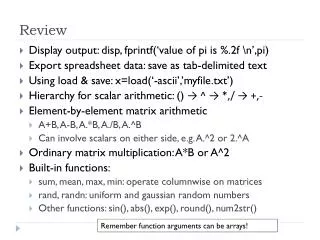
Review • Display output: disp, fprintf(‘value of pi is %.2f \n’,pi) • Export spreadsheet data: save as tab-delimited text • Using load & save: x=load(‘-ascii’,’myfile.txt’) • Hierarchy for scalar arithmetic: () → ^ → *,/ → +,- • Element-by-element matrix arithmetic • A+B, A-B, A.*B, A./B, A.^B • Can involve scalars on either side, e.g. A.^2 or 2.^A • Ordinary matrix multiplication: A*B or A^2 • Built-in functions: • sum, mean, max, min: operate columnwise on matrices • rand, randn: uniform and gaussian random numbers • Other functions: sin(), abs(), exp(), round(), num2str() Remember function arguments can be arrays!
Compute (using sum then without sum) • k=1:15; • sum(k.^2) • k*k' • Generate a vector r of means for 1000 random number vectors of length 50. • r = mean(rand(50,1000));
MATLAB Function Files • A MATLAB function file (called an M-file) is a text (plain ASCII) file that contains a MATLAB function and, optionally, comments. • The file is saved with the function name and the usual MATLAB script file extension, ".m". • A MATLAB function may be called from the command line or from any other M-file. • When the function is called in MATLAB, the file is accessed, the function is executed, and control is returned to the MATLAB workspace. • Since the function is not part of the MATLAB workspace, its variables and their values are not known after control is returned. • Any values to be returned must be specified in the function syntax.
TWO-DIMENSIONAL plot() COMMAND The basic 2-D plot command is: plot(x,y) • where x is a vector (one dimensional array), and y is a vector. Both vectors must have the same number of elements. • If the values of y are determined by a function from the values of x, than a vector x is created first, and then the values of y are calculated for each value of x. The spacing (difference) between the elements of x must be such that the plotted curve will show the details of the function.
x 1 2 3 5 7 7.5 8 10 y 2 6.5 7 7 5.5 4 6 8 PLOT OF GIVEN DATA Given data: >> x=[1 2 3 5 7 7.5 8 10]; >> y=[2 6.5 7 7 5.5 4 6 8]; >> plot(x,y) Once the plot command is executed, the Figure Window opens with the following plot.
plot(x,y,’line specifiers’) LINE SPECIFIERS IN THE plot() COMMAND • Line specifiers can be added in the plot command to: • Specify the style of the line. • Specify the color of the line. • Specify the type of the markers (if markers are desired).
plot(x,y,‘line specifiers’) LINE SPECIFIERS IN THE plot() COMMAND Line Specifier Line Specifier Marker Specifier Style Color Type Solid - red r plus sign + dotted : green g circle o dashed -- blue b asterisk * dash-dot -. Cyan c point . magenta m square s yellow ydiamond d black k
LINE SPECIFIERS IN THE plot() COMMAND • The specifiers are typed inside the plot() command as strings. • Within the string the specifiers can be typed in any order. • The specifiers are optional. This means that none, one, two, or all the three can be included in a command. EXAMPLES: plot(x,y) A solid blue line connects the points with no markers. plot(x,y,’r’) A solid red line connects the points with no markers. plot(x,y,’--y’) A yellow dashed line connects the points. plot(x,y,’*’) The points are marked with * (no line between the points.) plot(x,y,’g:d’) A green dotted line connects the points which are marked with diamond markers.
Line Specifiers: red line and asterisk markers. PLOT OF GIVEN DATA USING LINE SPECIFIERS IN THE plot() COMMAND >> plot(x,y,‘-r*')
Plotting: simple xy graphs Can further enhance line properties with: plot(x,y,’PropertyName’,value,...) For example: plot(x,y,'LineWidth',3.0) For log plots use: semilogy (x: linear, y:log) loglog (both log) It is possible to place more than one set of axes on a single figure, creating multiple subplots using subplot(m,n,p) This creates mxn subplots in the current figure. Subplots are then created row by row,
Subplots For example: • figure(1) • subplot(2,1,1) • x = -2:0.01:2; • y = x.^2; • plot(x,y) • subplot(2,1,2) • y = x.^3; • plot(x,y)
CREATING A PLOT OF A FUNCTION Consider: A script file for plotting the function is: % A script file that creates a plot of % the function: 3.5^(-0.5x)*cos(6x) x = [-2:0.01:4]; y = 3.5.^(-0.5*x).*cos(6*x); plot(x,y) Creating a vector with spacing of 0.01. Calculating a value of y for each x. Once the plot command is executed, the Figure Window opens with the following plot.
CREATING A PLOT OF A FUNCTION If the vector x is created with large spacing, the graph is not accurate. Below is the previous plot with spacing of 0.3. x = [-2:0.3:4]; y = 3.5.^(-0.5*x).*cos(6*x); plot(x,y)
THE fplot COMMAND The fplot command can be used to plot a function with the form: y = f(x) fplot(‘function’,limits) • The function is typed in as a string. • The limits is a vector with the domain of x, and optionally with limits of the y axis: [xmin,xmax] or [xmin,xmax,ymin,ymax] • Line specifiers can be added.
PLOT OF A FUNCTION WITH THE fplot() COMMAND A plot of: >> fplot('x^2 + 4 * sin(2*x) - 1', [-3 3])
PLOTTING MULTIPLE GRAPHS IN THE SAME PLOT Plotting two (or more) graphs in one plot: • Using the plot command. • 2. Using the holdon, hold off commands.
USING THE plot() COMMAND TO PLOT MULTIPLE GRAPHS IN THE SAME PLOT plot(x,y,u,v,t,h) • Plots three graphs in the same plot: • y versus x, v versus u, and h versus t. • By default, MATLAB makes the curves in different colors. • Additional curves can be added. • The curves can have a specific style by adding specifiers after each pair, for example: plot(x,y,’-b*’,u,v,’-ro’,t,h,’-g+’)
Plot of the function, and its first and second derivatives, for , all in the same plot. USING THE plot() COMMAND TO PLOT MULTIPLE GRAPHS IN THE SAME PLOT x = [-2:0.01:4]; y = 3*x.^3-26*x+6; yd = 9*x.^2-26; ydd = 18*x; plot(x,y,'-b',x,yd,'--r',x,ydd,':k') vector x with the domain of the function. Vector y with the function value at each x. Vector yd with values of the first derivative. Vector ydd with values of the second derivative. Create three graphs, y vs. x (solid blue line), yd vs. x (dashed red line), and ydd vs. x (dotted black line) in the same figure.
USING THE plot() COMMAND TO PLOT MULTIPLE GRAPHS IN THE SAME PLOT
Exercises Before you start, create a new file ex4_1.m in your home directory, then edit it to create the following as 2 horizontally arranged subplots: 1. Draw a graph that joins the points (0,1), (4,3), (2,0) and (5,-2) with each point as an asterisk. 2. Draw a target made up of three circular rings of radius 1, 2 and 3. The formula for the co-ordinates of a circle are: x = r.cos(θ) 0 < θ < 2π y = r.sin(θ) r > 0 You may need to use the command axis('equal‘).
USING THE hold on, hold off, COMMANDS TO PLOT MULTIPLE GRAPHS IN THE SAME PLOT hold on Holds the current plot and all axis properties so that subsequent plot commands add to the existing plot. hold off Returns to the default mode whereby plot commands erase the previous plots and reset all axis properties before drawing new plots. This method is useful when all the information (vectors) used for the plotting is not available at the same time.
Plot of the function, and its first and second derivatives, for all in the same plot. USING THE hold on, hold off, COMMANDS TO PLOT MULTIPLE GRAPHS IN THE SAME PLOT x = [-2:0.01:4]; y = 3*x.^3-26*x+6; yd = 9*x.^2-26; ydd = 18*x; plot(x,y,'-b') hold on plot(x,yd,'-r') plot(x,ydd,‘-k') hold off First graph is created. Two more graphs are created.
EXAMPLE OF A FORMATTED 2-D PLOT Plot title Legend y axis label Text Tick-mark Data symbol x axis label Tick-mark label
FORMATTING COMMANDS title(‘string’) Adds the string as a title at the top of the plot. xlabel(‘string’) Adds the string as a label to the x-axis. ylabel(‘string’) Adds the string as a label to the y-axis. axis([xmin xmax ymin ymax]) Sets the minimum and maximum limits of the x- and y-axes.
FORMATTING COMMANDS legend(‘string1’,’string2’,’string3’) Creates a legend using the strings to label various curves (when several curves are in one plot). text(x,y,’string’) Places the string (text) on the plot at coordinate x,y relative to the plot axes.
EXAMPLE OF A FORMATTED PLOT x=[10:0.1:22]; y=95000./x.^2; xd=[10:2:22]; yd=[950 640 460 340 250 180 140]; plot(x,y,'-','LineWidth',1.0) hold on plot(xd,yd,'ro-','linewidth',1.0) hold off Creating vector x for plotting the theoretical curve. Creating vector y for plotting the theoretical curve. Creating a vector with coordinates of data points. Creating a 2nd vector of data.
EXAMPLE OF A FORMATTED PLOT Formatting of the light intensity plot (cont.) xlabel('DISTANCE (cm)') ylabel('INTENSITY (lux)') title(‘Light Intensity','FontSize',20) axis([8 24 0 1200]) text(14,700,'Comparison between theory and experiment.') legend('Theory','Experiment')
Saving • Once your figure is ready you can save it as postscript (eps) • -- Function File: print () • -- Function File: print (OPTIONS) • -- Function File: print (FILENAME, OPTIONS) • -- Function File: print (H, FILENAME, OPTIONS) • Print a graph, or save it to a file • The device options “-dpdf” and “–depsc2” will save as PDF and EPS respectively.
Exercise • Create a new m-file “plotsin2.m” in your work directory • Plot f(x) = sin(2x) and its derivative f’(x) = 2cos(2x) on the same axes in the interval [0,2π]. Use the ‘hold on’ method. • Add axes labels and a title • Add a legend using legend(‘f(x)’,’d/dx f(x)’) • Note: For those of you familiar with LaTex, you can use some LaTex commands in title/legends, etc., e.g. title(‘time-course of \lambda’) • Save it to a PDF file.


