M82
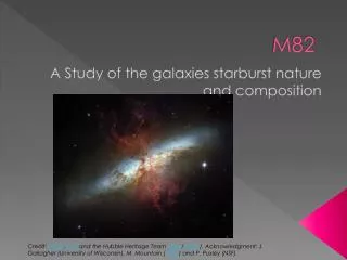
M82 . A Study of the galaxies starburst nature and composition. Credit: NASA , ESA and the Hubble Heritage Team STScI / AURA ). Acknowledgment: J. Gallagher (University of Wisconsin), M. Mountain ( STScI ) and P. Puxley (NSF). Basic Information.


M82
E N D
Presentation Transcript
M82 A Study of the galaxies starburst nature and composition Credit: NASA, ESA and the Hubble Heritage Team STScI/AURA). Acknowledgment: J. Gallagher (University of Wisconsin), M. Mountain (STScI) and P. Puxley (NSF).
Basic Information • M82, located in Ursa Major, was first discovered by Johann Elert Bode in 1774. • Its classified as a prototype Starburst Galaxy of the second type, famous for its heavy star formation due to its close encounter with its neighbouring galaxy M81. • M82 is five times as bright as the entire milky way galaxy, and 100 times as bright as the Mily Way’s center, although only about a quarter of its size.
Basic Information • Distance to Object: 11.5 +- 0.8 Mly • Size : • 10.47’ x 4.365’ (Angular Size) • (Physical Size) • Apparent Magnitude : 9.3 • Position: • (J200) RA: 09h 55m 52.2s D: +69° 40′ 47″
How to locate M82 • First locate the big dipper. The next step is to draw an imaginary line from gamma Ursae Majoris to alpha Ursae Majoris, then double its length in the same direction. • Doing this alone, you will most probably locate M81 as a very faint patch of light. M82 is located close by and is generally harder to locate as it has a low magnitude. This method may be summarized by the following diagram. Backyard Astro. 2009. Deepsky Top-100 (10): M 81 & M82. http://www.backyard-astro.com/deepsky/top100/10.html
Observing the Galaxy at different wavelengths • In X-ray • Chandra Telescope. • Credit NASA/SAO/G.Fabbiano et al. • Scale Image is 5 arcmin across. • Release Date June 05, 2001 • Red = low energy, green intermediate, and blue high-energy X-rays. White and yellow sources emit both low- and high-energy X-rays • Observation Time 13 hours • Observation Dates September 20, 1999 Frommert H, Kronberg C. 1998. The Messier Catalogue. http://seds.lpl.arizona.edu/Messier/more/m082_cxo.html The bright spots in the center are Supernova remnants or X-ray binaries. Observing M82 in the Infrared spectrum, it is the brightest galaxy in the sky.
Spitzer Telescope Image (Infrared) • Scale: 7.9 arcmins ac ross • Telescope : Spitzer Telescope • Image Credit: NASA/JPL-Caltech/C. Engelbracht (University of Arizona) • Instrument: IRAC • Wavelength: Infrared: Red • Exposure Date: May 6, May 8, and May 9 2005 • Exposure Time: 4 minutes per point, 1 hour for full image • Field of View: 12.6 x 12.6 arcminutes • Orientation: North is 57.7 deg counter clockwise from up • Release Date: 16 March 2006 Chandrea X-ray Observatory. 2008. http://chandra.harvard.edu/photo/2006/m82/more.html
ASTRO-1 UIT – UV spectrum • This picture was taken with a combination of telescopes: the VLA in New Mexico, and the MERLIN in the UK • The reason behind the three distinct maxima is most widely described by the presence of UV-absorbing dust covering its nucleus. Frommert H, Kronberg C. 1998. The Messier Catalogue. http://www.seds.org/messier/more/m082_uit.html
Astro-1 UIT - Visible • The image is in false colour • The dust covering the galaxies core is still visible, however, not as prominent as with the UV image taken with the same telescope Frommert H, Kronberg C. 1998. The Messier Catalogue. http://www.seds.org/messier/more/m082_uit.html
Multi-Wavelength Distribution • Credit: X-ray: NASA/CXC/JHU/D.Strickland; Optical: NASA/ESA/STScI/AURA/The Hubble Heritage Team; IR: NASA/JPL-Caltech/Univ. of AZ/C. Engelbracht • Scale: Image is 7.9 arcmin across • Observation Dates: June 18, 2002 • Observation Time: 5 hours • Color Code Energy : (X-ray: Blue; Optical: Green & Orange; Infrared: Red) • Instrument : ACIS • Release Date: April 24, 2006 Chandrea X-ray Observatory. 2008. http://chandra.harvard.edu/photo/2006/m82/more.html
Research Topic : Starburst Regions • A starburst galaxy is a galaxy in which there is an abnormal amount of star creation. • Two main types of Starburst Galaxies: • Blue Compact Galaxies • Contain low amounts of mass, metallicity, and dust, and contain a large amount of hot young stars. • Radiate in the UV spectrum • Ultra-luminous Infrared Galaxies • Generally extremely dusty. • Seen in the infrared. The UV light emitted from the hot young stars is absorbed and reemitted as infrared by the dust flooding the galaxy. • The center of a ULIRG can be seen in the X-ray spectrum.
Starburst Galaxies • In order to create a Starburst Galaxy, there must be present a large supply of gas to form large amounts of new stars. This large amount of gas must undergo compression through tidal forces triggered by a close encounter or collision with another nearby galaxy • M82’s high level of star formation is due to a close encounter with its neighbouring galaxy M81. The interaction is evident through discovery of large streams of neutral hydrogen connecting the two galaxies seen in the radio spectrum.
“What can be understood upon observing M82’s UV radiation?” • Far-UV imaging of the starburst galaxy M82 • One of the maxima is interpreted to be a reflection nebula, and the other two due to massive stars in gas and dust poor locations in the outer disk. • They used two telescopes, • SCAP with a diameter of 13 cm • FOCA with a diameter of 40 cm. • M82 was observed using FOCA, which was mounted to a balloon that rose to 40 km altitude and is sensitive to wavelengths between 195 nm and 210 nm. They took 8 exposures of 150s each covering a field of view of 2.3 degrees, centered on 9h 58m 57.0 s, +69 degrees 01’ 41”.
“What can be understood upon observing M82’s UV radiation?” • The central region was found to have a minimum connecting the two maxima (in the form of a saddle point in the 2D image). • The central region is therefore not a maximum of UV emission, as expected • They conclude that the regions of high UV emission have an absence of IR, and therefore gas and dust poor. • One possible explanation for the UV emission is the presence of very hot burning stars in dust and gas poor regions . • The presence of two distinct regions may either mean that there exists two distinct emission regions or that absorbing matter is located infront of the plane in the central regions
Taking the images and Processing our Data • The telescope used to take our images was the 40 cm Evan’s reflecting telescope at the Glenlea Observatory in Winnipeg Manitoba. • An apogee AP-47 CCD camera was used for capturing the images. • We used ImageJ for processing our images and developing a final processed image of the galaxy M82
Master Bias • Convert the images to 32 bit. • Measure the mean value of the over scan region for each Bias Frame image used via analyze>Set Measurements>”check mean grey values”, then Analyze>Measure. • This is a region of size 6 x 512 pixels along the left hand side of each image. • Remember to open each group of images as a Stack and to use to ROI Manager to manage each image in the stack. • Subtract this mean pixel value from each of the bias frames, then crop each image to 520 x 512. • The Master Bias frame is the average of 10 bias frames, and can be created with the use of the ROI manager and Z project
Master Bias • Raw Data: • Date: Feb. 08, 2007 • Time: 7:16 – 7:18 PM • Temperature: -29 °C • CloudCover: Clear • Moon: Wanning Gibbous • Visibility: 22.7 km • Equipment: The 40 cm Evans' reflecting telescope • Size : 520 x 512
Master Dark • To Create a Master Dark, subtract the over scan region and crop as done with the Master Bias region. Further, subtract the Master Bias frame from each Dark Frame via Process>Math>Subtract. (Remember everything must be in 32 bit format) • Z stack the Dark frames to create the final Master Dark frame.
Master Dark • Raw Data • Date: Feb. 08, 2007 • Time: 7:25 – 7:51 PM • Temperature: -29 °C • CloudCover: Clear • Moon: Waning Gibbous • Visibility: 22.7 km • Equipment: The 40 cm Evans' reflecting telescope • Size : 520 x 512 • Exposure time: 300s
Dark Sky Flats • To create the Master Flat frame (in our case Dark Sky Flats), first convert the images to 32 bit format, subtract the over scan region, crop to 520 x 512 pixel size, and subtract both the Master bias frame and Master Dark frame from each image. • Because the stars appear in different locations from image to image, we may make use of the plug-in called “Background Extractor” which will normalize the sky frames and create the final Master Flat image. ( Normalize each image by Mean, and Combine stack by Median)
Dark sky flats • Raw Data: • Date: Feb. 08-09, 2007 • Time: 11:39 – 12:03 PM • Temperature: -29 °C • CloudCover: Clear • Moon: Wanning Gibbous • Visibility: 22.7 km • Equipment: The 40 cm Evans' reflecting telescope • Size : 520 x 512 • Exposure time: 300 s • Comments; The dust halos are quite evident.
The final dark-subtracted, flat-fielded and co-added but otherwise unmanipulated image. • We must first convert the images to 32-bit format, subtract the overscan region from each image, crop each image to 520 x 512 pixel size, subtract the master bias frame from each image, subtract the master dark frame from each image, and finally divide each image by the master flat. • Select the usable frames, and register and combine them via the set of plug ins “TurboReg” and “StackReg” to register and aligned the frames, • We now have the final image of our Galaxy!
Our image of M82 • Raw data • Date: Feb. 08 2007 • Time: 10:58 – 11:31 PM • Temperature: -29 °C • CloudCover: Clear • Moon: Wanning Gibbous • Visibility: 22.7 km • Equipment: The 40 cm Evans' reflecting telescope • Size : 520 x 512 • Exposure time: 300s each
Finding the field of view of our images • To find the field of view for our images, we may use an image of the “double double” star Eplison Lyrae. • Plotting a Profile across both stars will lead us to a separation in pixels between the two stars, and knowing the true distance between them can allow us to develop a scale by which we may calculate the angular field of view for our images.
Field of View • We find:
Pixel Counts of certain regions of our image: • Background Sky: • Three value average: • 1856.26, 1982.14, 1914.34 • Average : 1917.58
Pixel Counts of certain regions of our image: • Faintest observable region of the object • Outer extension of M82 to the left: • 2467.82, 2334.34, 2300.34 • Average: 2367.5 +- 80.0 • Outer extension of M82 to the right: • 2309.34, 2359.56, 2488.45 • Average: 2385.79 +- 90.00
Pixel Counts of certain regions of our image: • Brightest region of the object: the galaxies core • Plotting the pixel profile of a 10 pixel radius around the core, we find that its peak pixel value is : 14479.12
Stellar Magnitudes • For Stellar bodies, I used the circle tool to analyze our image. The circle has a radius of 8 pixels (the size of the largest star). • Peak pixel value of faintest stellar object • The peak value for the faintest star : 2222.737
Peak pixel value of the brightest unsaturated stellar object • Peak pixel value of the brightest unsaturated stellar object: 64203.707 (note : this is now closely approaching the saturation limit)
Stellar Magnitudes • The stellar body is actually a cluster of millions of stars associated with M82. I used the circle tool to determine the flux through a circle of 8 pixel radius for each stellar body. • For the brightest stellar region, • IntDen : 5710094.058 • For the faintest stellar region, • IntDen: 403256.245 • The ratio of these values is : • 14.160 • To estimate the magnitude of the faint star, we can use the following equation: • Where m is the magnitude of the faint star. • The faint star therefore can be estimated to have a magnitude of m = 12.88.
Best Image for observing faint objects • Best image using linear scaling to easily observe faint regions of image. • This image was inverted via image>look up tables>Invert LUT • The image’s brightness and contrast was also altered • The surrounding dim stars may be more easily seen this way.
Best Image for observing faint objects • Using : • Image>look up tables>royal • Image>look up tables >invert LUT • The following image can be determined. • In this image, the brightest parts of the core of the galaxy may be seen in more detail.
Another method by which the bright regions of M82 can seen: • Using: • Image>look up tables>phase • In this image, the regions closely surrounding the nuclear regions are detailed. One can clearly see the edges of this region. This image is of false colour.
A logarithmically scaled image: • Changing the transfer function to a logarithmic one will reduce saturation as well as increase the detail of the brighter regions of our galaxy. • The image was obtained by Process>Math>Log in ImageJ
Contour Mapping • A Contour mapping of the image will show associations between different regions. • These are the pixel values by which the boundaries may be calibrated. • We used the following settings:
The associated Contour Map of M82 • I set the outer green boundary to a pixel value, 2300 , within error of the values found earlier for the outer edge of the visible galaxy. • Orange : the boundary in which the bright white region which makes up the body of the galaxy • Red: the apparent multi-core nature of the galaxy in the visible spectrum • Blue: the brightest of these ‘cores’ (the true nucleus).
Plotting Pixel Profile across certain regions of our image Dimmest Stellar Body has a typical Gaussian shaped distribution curve
Across Galaxy • From this plot, the large amount of enveloping dust and gas around M82’s core is most evident. It may be associated with the large dips in the luminosity distribution. • This profile plot cannot be associated with a Gaussian curve. • Due to perhaps the large amount of dust covering its center, a large dip in the profile may be seen.
Examining the apparently multi-cored nature at M82’s center • Examining the bridge between the apparent core and the associated bright region to the left of the nucleus, one can more clearly see the distinction between the two peak brightness values, and perhaps the presence of dust and gas covering one single bright region. Then it was scaled to ten times larger. Also, it was : image>Look up Tables>Phase. Finnaly it was sharpened.
Estimating the Angular size of our Galaxy • We may use our calculated field of view and the boundary defined through our contour mapping to determine the angular size of our galaxy. Measured across and length wise: • Its length is: 19.1 +- 0.1 cm • Its width is: 5.5 +- 0.1 cm • The width of the whole image is: 23.4 +- 0.2 cm (error double because measured by moving ruler once) • The estimated angular length is : (19.1 +- 0.1 cm / 23.4 +- 0.2 cm) x = (5.66 +- 0.30 arcmins) • The estimated angular width is : (5.4 +- 0.1 cm / 23.4 +- 0.2 cm) x = (1.60 +- 030 arcmins) • The expected angular size: 10.47’ x 4.365’ • Deviation due to the definition of our galaxies outer boundary.
Estimating Physical Size • Estimating our Physical size, we know: • (Distance to object) x tan (angular size) = (physical size of object) • Length : (11.5 +- 0.8 Mly) x tan ((5.66 +- 0.30) / (60) deg) = 18933.93 +- 2000.00 ly • Width: ((11.5 +- 0.8 Mly) x tan ((1.60 +- 0.30) / (60) deg)) = 5352.34 +- 1000.00 ly • As expected, these values are mathematically inconsistent with the known values of : • Actual size: (Physical Size) • This again has to do with the boundaries by which the size of the galaxy is defined.
Images from SLOAN digital sky survey • The spectral classification of each image is described by the following chart:
Top Left : U Top Right: G Middle : R Bottom Left: I Bottom Right: Z
SLOAN images • As expected, the dust and gas covering the center of the Galaxy grows less visible as the wavelength of light used to observe M82 increases. • Because the dust and gas absorbs the UV radiation emitted by the hot young stars from the Starburst regions of the galaxy, the dust is more visible upon viewing of the galaxy at smaller wavelengths (closer associated with the UV spectrum ) . Remember that the dust is represented by an absence of emission in the UV spectrum. (dark clouds)
Conclusion: • The galaxy I researched was M82, a prototype Starburst Galaxy famous for heavy star formation due to its close encounter with M81. • Through the use of several image processing techniques including general image reduction with the use of the • Master Bias, • Master Dark, • Master Flat • And the use of several more advanced processing techniques including • using look up tables>(invert LUT, royal, phase) • logarithmic image scaling • image sharpening • manipulation of the brightness and contrast, • Through these methods we could more easily analyze our image.
Conclusion • We found that in correlation to past research in the UV emission spectrum, the dust was more visible (an absence of emission) as dark clouds surrounding the center of the galaxy. Wilson and Petipas were able to determine that the double peaked nature could also be due to the result of two individually separated clumps of molecular gas collecting on a inner Lindblad resonance (ILR) and not an edge on molecular torus. • We determined a physical and angular size of our galaxy, however our results were not consistent with the expected ones
References Barker S., de Grijs R, Cerviño M, 2008. Star cluster versus field star formation in the nucleus of the prototype starburst galaxy M 82. Astrophys J 484(3): 711 Backyard Astro. 2009. Deepsky Top-100 (10): M 81 & M82. http://www.backyard-astro.com/deepsky/top100/10.html Cotton WD, Condon JJ, Arbizzani E. 1999. Arcsecond positions of UGC galaxies. Astrophys J 125:409 Courvoisier TJL, Reichen, M, Blecha, A, Golay M, Huguenin D. Far-UV imaging of the starburst galaxy M82. Astrophys J 238(1): 63 Frommert H, Kronberg C. 1998. The Messier Catalogue. http://www.seds.org/messier/more/m082_uit.html Marcia R. 2008. http://ircamera.as.arizona.edu/astr_250/Lectures/Lec_24sml.htm McKeith CD, Castles J, Greve A, Downes D. 1993. Rotation of Stars and Gas in M82. Astrophys J 22 (1):98
References Moor JH, Smith L, Westmoquette M, 2004. Starburst Galaxy Showers The Universe. http://zuserver2.star.ucl.ac.uk/~msw/M82_pr/ Peach D. 2004. Binaries. http://www.damianpeach.com/binaries.htm Petitpas GR, Wilson CD, 1999. Dynamics, Distribution, and Amount of Molecular Gas in Galaxies with NIR Isophote Twists: NGC 2273 & NGC 5728. Cassiopeia Online September 1999 issue : 102 Petitpas GR, Wilson CD, 2000. TemperatureandDensityGradientsAcrosstheNucleusofM82. Astrophys J 538: 117 Thaller M, Doris D, Hermans-Killam L, Hurt R. 2008. Multi Wavelength Astronomy. http://coolcosmos.ipac.caltech.edu/cosmic_classroom/multiwavelength_astronomy/multiwavelength_museum/m82.html The 8th European VLBI Network Symposiumon New Developments in VLBI Science and Technologyand EVN Users Meeting. 2006. www.astro.uni.torun.pl/evn2006/presentation/Tom_Muxlow.ppt The Internet Encyclopedia of Science. 2008. Starburst Galaxy. http://www.daviddarling.info/encyclopedia/S/starburst_galaxy.html Wikipedia. Epsilon Lyrae. http://en.wikipedia.org/wiki/Epsilon_Lyrae Wikpedia. Starburst Galaxy. http://en.wikipedia.org/wiki/Starburst_galaxy