Download
1 / 21
220 likes | 544 Vues
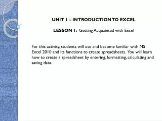
UNIT 1 – INTRODUCTION TO EXCEL LESSON 1: Getting Acquainted with Excel For this activity, students will use and become familiar with MS Excel 2010 and its functions to create spreadsheets. You will learn how to create a spreadsheet by entering, formatting, calculating and saving data.

E N D
UNIT 1 – INTRODUCTION TO EXCEL LESSON 1: Getting Acquainted with Excel For this activity, students will use and become familiar with MS Excel 2010 and its functions to create spreadsheets. You will learn how to create a spreadsheet by entering, formatting, calculating and saving data.
Double click on the MS Excel 2010 icon located on the desktop.
Use the “drop down arrow” to save your document onto your USB Drive.
In the “File Name” option type: your First Name_LastName_Activity One. For example Sheri_Lundrigan_Activity One.
Enter the following data as seen below between the quotation marks. • You can use your mouse to click into each individual cell or use the arrow keys on your keyboard to move from cell to cell. • Type “PROJECT COST CONTROL SPREADSHEET” in Cell A1 • Type “BUDGET” in Cell B3 • Type “ACTUAL” in Cell C3 • Type “$ DIFFERENCE” in Cell D3 • Type “Software” in Cell A5 • Type “Hardware” in Cell A6 • Type “Office Supplies” in Cell A7 • Type “Travel” in Cell A8 • Type “Labour” in Cell A9 • Type “Delivery Costs” in Cell A10 • Type “Telephone” in Cell A11 • Type “Advertising” in Cell A12 • Type “Postage” in Cell A13 • Type “TOTAL EXPENSES” in Cell A15
You will notice that some of your text has entered into another cell. To fix this, we have to adjust the column width.
Selecting Ranges: Practice using this technique by holding your left mouse button to select and highlight a range (block) of cells. Click Row 3 and while holding the button down on your mouse, slide it down to Row 15.
Time to format the size of the cells. To do this, click the “Home” tab on the “Tab List” and then the “Format” button on the “Ribbon” Tab List Ribbon
Type “1500” in cell B5 Type “3000” in cell B6 Type “350” in cell B7 Type “200” in cell B8 Type “9000” in cell B9 Type “600” in cell B10 Type “450” in cell B11 Type “700” in cell B12 Type “100” in cell B13 Type “1295” in cell C5 Type “3250” in cell C6 Type “457” in cell C7 Type “173” in cell C8 Type “9750” in cell C9 Type “582” in cell C10 Type “496” in cell C11 Type “894” in cell C12 Type “85” in cell C13 For Cell D5 key in the following formula “=SUM(B5-C5)” and hit you enter key. Copy and paste Cell D5 into cells D6 through to D13.
Formatting Cells: Select to highlight Cells A1, B3, C3 and D3 and format the headings bold by selecting the “B” on the “Ribbon”
Select to highlight cells B5 through to B13 along with C5 through to C13 and D5 through to D13 and change the numbers to currency by clicking the “$” button on the Ribbon.
NOTE: You may have to adjust the width of your columns again several times (like you did in the steps above). To format the size of the cells you have to select the cells to highlight them and then click the “Home” tab on the “Tab List” and then the “Format” button on the “Ribbon” and select “AutoFit Column Width”
Enter the following formula in cell B15 “=SUM(B5:B13)” Enter the following formula in cell C15 “=SUM(C5:C13)” Enter the following formula in cell D15 “=SUM(D5:D13)” (Re-Adjust Column Width) Select to highlight cells B15, C15 and D15 to place a line on top and a double line on bottom of those cells by clicking the “Top and Double Bottom Border” on the ribbon.
Bold Cell A15 and then your spreadsheet should look like the one below
Click the “Save” button on the “Quick Access Toolbar” Quick Access Toolbar
Note: To close window, click the lower “x”. If you click the upper “x”, you will exit the MS Excel Program. Students should also be reminded to save their work frequently by clicking the quick save button. Close Program Button Clos Close Window Button Window Button