Syntactic Analysis and Parsing Techniques: A Comprehensive Guide
420 likes | 693 Vues
Learn how compilers transform source code through phases, particularly focusing on Syntax Analysis or Parsing, including top-down and bottom-up methods. Explore predictive parsers, handling left-recursive grammars, and more.

Syntactic Analysis and Parsing Techniques: A Comprehensive Guide
E N D
Presentation Transcript
Syntactic Analysis and Parsing Based on A. V. Aho, R. Sethi and J. D. Ullman Compilers: Principles, Techniques and Tools
Compilers • A compiler is an application that reads a program written in the source language and translates it into the target language. • A compiler operates in phases. Each phase transforms the source program from one representation to another. Source program Lexical Analyzer Syntax Analyzer Semantic Analyzer Intermediate Code Generator Code Optimizer Code Generator Target Program • The part of the compiler on which we will focus here is the Syntax Analyzer or Parser.
Parsing • Parsing determines whether a grammar can generate a string of tokens. It builds a parse tree. • Most parsing methods fall into one of two classes: top-downand bottom-up methods. • In top-down parsing, construction starts at the root and proceeds down to the leaves. In bottom-up parsing, construction starts at the leaves and proceeds up towards the root. • Efficient top-down parsers are easily built by hand. • Bottom-up parsing, however, can handle a larger class of grammars. They are not as easy to build, but there are tools that generate parsers directly from a grammar.
Part I: Top-Down Parsing Points: • Basic ideas in top-down parsing • Predictive parsers • Left-recursive grammars • Left-factoring a grammar • Constructing a predictive parser • LL(1) grammars
Basic Idea in Top-Down Parsing • Top-Down Parsing is an attempt to find a left-most derivation for an input string • Example: S c A d Find a derivation for A a b | a for w c a d S Sbacktrack S / | \ / | \ / | \ c A d c A d c A d / \ | a b a
Predictive Parsers: Generalities • In many cases, careful writing – left recursion eliminated and left-factoring considered – we can get a grammar that parses using recursive descent, and needs no backtracking. • Such parsers are called predictive parsers.
Left Recursive Grammars (1) • A grammar is left-recursive if it has a non-terminal A such that for some string α there is a derivation A A α • A top-down parser can loop when it faces a left-recursive rule. Therefore, such rules must be eliminated. • As an example, the left-recursive rule A A α | β can be replaced by: • A β R where R is a new non-terminal • R α R | and is the empty string • The new grammar is right-recursive.
Left-Recursive Grammars (2) • Here is the general procedure for removing direct left recursion that occurs in one rule: • Group the A-rules like this: A A α1 |… | A αm | β1 | β2 |…| βn where no β begins with A. • Replace the original A-rules with • A β1 A’ | β2 A’ | … | βn A’ • A’ α1 A’ | α2 A’ | … | αm A’ | • This procedure will not eliminate indirect left recursion of the kind: • A B a A • B A b [There is another procedure (we will skip it).] • Direct or indirect left recursion is problematic for all top-down parsers. It is not a problem for bottom-up parsing algorithms.
Left-Recursive Grammars (3) Here is an example of a (directly) left-recursive grammar: E E + T | T T T * F | F F ( E ) | id This grammar can be re-written as the following not left-recursive grammar: E T E’ E’ + T E’ | T F T’ T’ * F T’ | F ( E ) | id
Left-Factoring a Grammar (1) • Left recursion is not the only property that hinders top-down parsing. • Another difficulty is the parser’s inability always to choose the correct right-hand side on the basis of the next input token. The idea is to consider only the first token generated by the leftmost non-terminal in the current derivation. • To ensure it, we need to left-factor formerly left-recursive grammars – as the one generated in the preceding example.
Left-Factoring a Grammar (2) The procedure of left-factoring a grammar • For each non-terminal A, find the longest prefix α common to two or more of its alternatives. • The A productions are as follows: A α β1 | α β2 … | α βn | ( denotes all alternatives that do not begin with α) • Replace that with: A α A’ | A’ β1 | β2 | … | βn
Left-Factoring a Grammar (3) • Here is an example of a well-known grammar that needs left-factoring: S if E then S | if E then S else S | a E b • Left-factored, this grammar becomes: S if E then S S’ | a S’ else S | E b
Predictive Parsers: Details • The key problem during predictive parsing: determine the production to be applied to a non-terminal. • This is done using a parsing table. • A parsing table is a two-dimensional array M[A, ] where A is a non-terminal, and is either a terminal or the symbol $ that denotes the end of input string. • Other data for a predictive parser: • The input buffer contains the string to be parsed, followed by $. • The stack contains a sequence of grammar symbols; initially, it is $S (end of the input string and the grammar’s start symbol).
Predictive Parsers: Informal Procedure • The predictive parser considers X, the symbol on the top of the stack, and , the current input symbol. It uses the parsing table M. • X = = $ stop with success • X = ≠ $ pop X off the stack and advance the input pointer to the next symbol • X is a non-terminal check M[X, ] • If the entry is a production, then pop X and push the right-hand side of this production (one by one) • If the entry is blank, then stop with failure
Predictive Parsers: an Example Parsing Table Parsing Trace
Constructing a Parsing Table (1): First and Follow First(y) is the set of terminals that begin the strings derived from y. Follow(A) is the set of terminals that can appear to the right of A. First and Follow are used in the construction of the parsing table. To compute First: • X is a terminal First(X) = {X} • X is a production add to First(X) • X is a non-terminal and X Y1 Y2 … Yk is a production place z in First(X) if z is in First(Yi) for some i and is in all of First(Y1) … First(Yi-1)
Constructing a Parsing Table (2): First and Follow To compute Follow • Place $ in Follow(S), where S is the start symbol and $ is the end-of-input marker. • There is a production A B β everything in First(β) except for is placed in Follow(B). • There is a production A B, or a productionA B β where First(β) contains everything in Follow(A) is placed in Follow(B)
Constructing a Parsing Table (3): First and Follow, an Example E T E’ E’ + T E’ | T F T’ T’ * F T’ | F ( E ) | id First(E) = First(T) = First(F) = {(, id} First(E’) = {+, } First(T’) = {*, } Follow(E) = Follow(E’) = {), $} Follow(F) = {+, *, ), $} Follow(T) = Follow(T’) = {+, ), $}
Constructing a Parsing Table (4) An algorithm for constructing a predictive parsing table for a grammar: • For each production A , do steps 2 and 3 • For each terminal t in First(), add A to M[A, t] • If is in First(), add A to M[A, t] for each terminal t in Follow(A). If is in First() and $ is in Follow(A), add A to M[A, $]. • Mark each undefined element of M as an error.
LL(1) Grammars • A grammar whose parsing table does not contain multiply-defined entries is said to be LL(1). • No ambiguous grammar and no left-recursive grammar can be LL(1). • A grammar is LL(1) iff for any pair of productions A and A β the following conditions hold: • there is no terminal t for which both and β derive strings beginning with t • at most one of and β can derive the empty string • if β can (directly or indirectly) derive , then does not derive any string beginning with a terminal in Follow(A)
Part II: Bottom-Up Parsing • One of several methods of bottom-up syntactic analysis is Shift-Reduce parsing. It has several different forms. • Operator-precedence parsing is such form;another, much more general, is LR parsing. • In this presentation, we will look at LR parsing. It has three varieties. • Simple LR parsing (SLR) is an efficient but restricted version. • Canonical LR parsing is the most powerful, but also most expensive version. • LALRis intermediate in cost and power. Our focus will be on SLR Parsing.
LR Parsing: Advantages Warning: advertisement • LR parsers recognize any language for which a context-free grammar can be written. • LR parsing is the most general non-backtracking shift-reduce method known, yet it is as efficient as other shift-reduce algorithms. • The class of languages that can be parsed by an LR parser is a proper superset of what can be parsed by a predictive parser. • An LR-parser can detect a syntactic error as early as possible during a left-to-right scan of the input.
LR Parsing:Downside (easily prevented) • It is a lot of work to construct an LR parser by hand for a typical grammar of a programming language. • But: there are specialized tools that build LR parsers automatically. • With such tools, one must write a precise context-free grammar. From it, a parser generator automatically produces a parser for the underlying language. • An example of such a tool is Yacc – Yet Another Compiler-Compiler.
LR Parsing Algorithms: Details (1) • An LR parser consists of an input, output, a stack, a driver program and a parsing table. • The driver program is the same for all languages parsed. Only parsing tables differ. • The stack stores a sequence of the form s0 X1 s1 X2 … Xm sm(sm is at the top of the stack, s0 at the bottom). sk is a state symbol, Xi is a grammar symbol. Together, state and grammar symbols determine a shift-reduce parsing decision.
LR Parsing Algorithms: Details (2) • The parsing table, indexed by states and grammar symbols, has two parts. They define a parsing action function and a goto function. • The LR parsing program determines sm, the state on top of the stack, and ai, the current input token. In action[sm, ai] there can be one of four values: • Shift • Reduce • Accept • Error
LR Parsing Algorithms: Details (3) • action[sm, ai] = Shift s (s is a state) the parser pushes ai and s on the stack. • action[sm, ai] = Reduce A β A replaces a sequence that “covers” β. [hand-waving]Let the state now right below A in the stack be s. The value in goto[s, A] is a state: we push it onto the stack over A. • action[sm, ai] = Accept parsing succeeds • action[sm, ai] = Error
LR Parsing Example: The Grammar • E E + T • E T • T T * F • T F • F (E) • F id The numbers i-vi will appear in Reduce actions in the table.
SLR Parsing • Definition An LR(0) item of grammar G is a production of G with a dot inserted into the right-hand side. • Example From A X Y Z we can get four items: A . X Y Z A X . Y Z A X Y . Z A X Y Z . • Production A generates only one item, A . • Intuitively, the dot in an item shows how much of a production we have already seen at a given moment in the parsing process.
SLR Parsing • To create an SLR Parsing table, we define three new elements: • an augmentation of the initial grammar G. We add the production S’ . S where S is the start symbol of G. This new starting production will tell the parser when it should stop and accept the input. • the closure operation • the goto function
SLR Parsing:The Closure Operation Let W be a set of productions. We construct closure(W) by applying two rules. • Every production in W is added to closure(W). • If A . B is in closure(W) and B is a production, then add B . to W, if it is not already there. We apply this rule until no more new items can be added to closure(W).
SLR Parsing:The Closure Operation – Example Added production 0. E’ . E 1. E E + T 2. E T 3. T T * F 4. T F 5. F ( E ) 6. F id The original grammar Let W initially be {E’ . E}. Closure(W) = { E’.E, E.E+T, E.T, T.T*F, T.F, F.(E), F.id }
SLR Parsing:The Goto Operation • goto(W, X), where W is a set of items and X is a grammar symbol, is defined as the closure of the set of all items A X . B such that A . X B is in W. • Example: if W is {E E . + T, E’ E .}, then goto(W, +) contains E E + .T T . T * F T . F F . ( E ) F . id
SLR Parsing:Sets-of-Items Construction procedure items(G’) C = {Closure({[S’ .S]})} repeat for each set of items W in C and each grammar symbol X such that goto(W, X) is not empty and not in C do add goto(W, X) to C until no more sets of items can be added to C
Example: The Canonical LR(0) collectionfor grammar G’ W0: E’ . E E . E + T E . T T . T * F T . F F . ( E ) F . id W1: E’ E . E E . + T W2: E T . T T . * F W3: T F . W4: F ( . E ) E . E + T E . T T . T * F T . F F . ( E ) F . id W5: F id . W6: E E + . T T . T * F T . F F . ( E ) F . id W7: T T * . F F . ( E ) F . id W8: F ( E . ) E E . + T W9: E E + T . T T . * F W10: T T * F . W11: F ( E ) .
Constructing an SLR Parsing Table • Construct C = {W0, W1, … Wn}, the collection of sets of LR(0) items for G’. • State i is constructed from Wi. The parsing actions for state i are determined as follows: Wi contains A . t and goto(Wi, t) = Wjaction[i, t] = “Shift j”. Here, t must be a terminal. Wi contains A . action[i, t] = “Reduce A t”for all t in Follow(A). Here A may not be S’. Wi contains S’ S . action[i, $] = “Accept” If any conflicting actions are generated by the above rules, we say that the grammar is not SLR(1). The algorithm then fails to produce a parser.
Constructing an SLR Parsing Table (continued) 3. The goto transitions for state i are constructed for all nonterminals A like this:if goto(Wi, A) = Wj, then goto[i, A] = j. 4. All entries not defined by rules (2) and (3) are set to “Error”. 5. The initial state of the parser is the one constructed from the set of items containing S’ S . This requires practice...