Download
1 / 43
430 likes | 544 Vues
Ecosystem intercomparison between Nordic Seas and NW Atlantic. US PIs: G. Lough, L. Buckley, D. Mountain, M. Fogarty, T. Durbin, C. Werner Norwegian counterparts: S. Sundby, P. Budgell, Ø. Fiksen, E. Svendsen, V. Lien, T. Kristiansen

E N D
Ecosystem intercomparison between Nordic Seas and NW Atlantic US PIs: • G. Lough, L. Buckley, D. Mountain, M. Fogarty, T. Durbin, C. Werner Norwegian counterparts: • S. Sundby, P. Budgell, Ø. Fiksen, E. Svendsen, V. Lien, T. Kristiansen Objective: Develop an understanding of the processes controlling recruitment of cod and haddock on Georges Bank and cod in the Norwegian Sea sufficient to parameterize useful recruitment models and to forecast likely changes in abundance under a range of climate change scenarios. Modeling approach: • Global ROMS model run in Norway • Subsequently downscaled to NW Atlantic • Individual based models
Fig. 1. Atlantic cod distribution and spawning areas. Mean annual isotherms (oC) are indicated (Sundby, 2000).
Figure 2. Left (a): Schematic for the Georges Bank cod spawning and larval and juvenile drift (Lough and Manning, 2001), and right (b): as in (a) but for the Norwegian Shelf/Barents Sea (Vikebø et al. 2005).
High ambient temperature Tidally induced turbulence Weakly stratified by May due to solar insolation Diel light cycle 11-17h Significant offshore larval loss GB cod mature age 2-3 Vertical distribution different due to egg buoyancy, mixing Principal prey Pseudocalanus, Oithona spp. Advection of prey from Gulf of Maine Adult diet varied Low ambient temperature Wind induced turbulence NwCC strongly stratified due to freshwater runoff Continuous light end of May Minimal larval loss A-N cod mature age 6 Vertical distribution different due to egg buoyancy, mixing Principal prey Calanus finmarchicus Advection of Calanus from Norwegian Sea to Barents Sea Adult diet depends on Capelin Georges Bank vs Barents Sea
Hypotheses for the NW Atlantic and Norwegian Sea Systems • Hypothesis 1: strong and early influx of Scotian Shelf water to GOM leads to an early phytoplankton boom with increased zooplankton abundance downstream to Georges Bank resulting in increased larval cod/haddock growth. • Hypothesis 2: Advection of warm, zooplankton-rich Atlantic water from the Norwegian Sea onto the shelves (Barents Sea) results in increased larval cod growth and survival.
Collaborative Implementation • Modeled basin-scale circulation fields with increased resolution within the regional domains of the two ecosystems • Lagrangian (particle tracking) models for application within the regional domains • Individual-based trophodynamic models for larval and early juvenile fish growth to be embedded in the regional circulation models • Hybrid (full life-cycle) recruitment models that build on results and understanding gained from the detailed process studies and biophysical models
Fig. 3. Interannual changes in the seasonally averaged, normalized deviations for Georges Bank mean total abundance for each copepod taxa from the seasonally averaged 5-year mean (Durbin and Casas, 2005).
Fig. 4. Georges Bank data showing inter-annual variability between years with all abundant copepod taxa showing similar trends (Durbin and Casas). Both the chlorophyll changes and abundance changes were negatively correlated with salinity.
Fig 5a. Salinity variability on Georges Bank (0-30m) (bars, left axis, PSU) versus the distance of the north wall of the Gulf Stream (GS) from the shelf break in the Middle Atlantic Bight (solid line, right axis, km). A one-year smoothing was applied to the north wall series (T. Rossby, pers. comm). Note that the salinity series leads the GS series by about 6 to 8 months.
Fig 5b. The annual weighted average gadid (cod and haddock combined) early larval mortality rate (% per day) versus salinity anomaly for the five years of Georges Bank GLOBEC (Mountain et al. 2006). Low mortality with low salinity (and high zooplankton and high larval growth).
Fig 7a (left). Seasonal growth of 7mm cod larvae. Fig 7b (right). Interannual growth of 7mm cod larvae – hatching on 1 April (Buckley et al. 2005).
Fig. 8a (left). Prey for a 7 mm cod larvae. Values are monthly means for March to May ’95-99. Fig. 8b (right). Residual growth of a 7 mm cod larvae. Monthly means as in Fig. 8a. (Buckley and Durbin, 2005).
Larval Fish Trophodynamic Model Lough et al. 2005. Fish. Oceanogr. 14:4, 241-262
Selected Years of EmphasisNW Atlantic/ Georges Bank • The 1998 field season recorded minimum salinity due to the intrusion of Labrador Slope Water which was observed in the Northeast Channel and eventually came on to Georges Bank from the Gulf of Maine. High Calanus abundance also was noted that year from the broadscale surveys, as well as high haddock survival. • The 1999 season was warmer, more stratified, and an earlier Calanus bloom was noted which may have led to a 3rd generation (Durbin et al. 2003). Contrasting 1999 with 1998, where haddock survival also was high, will serve to check the hypotheses relating recruitment to secondary production. • The 1995 season had low haddock and cod survival during a warm year where Scotian Shelf intrusion was observed in March and the shelf/slope front moved on-bank to the 60-m isobath during May. What effect did these large physical events have on the residing populations?
Fig. 9. Snapshot SST (oC) for 1 January 1994 over the model domain implemented at IMR (P. Budgell, pers. comm.). The black rectangles are approximate domains of interest for the NW Atlantic (see Fig. 10 detail) and the Norwegian/Barents Seas. Axes are in arbitrary units.
Figure 10. Interannual variability of surface salinity (left column) and diatoms (right column) for February1995 (top row) and February 1999 (bottom row). Note the low salinity and early diatom bloom in the Georges Bank area in 1999 relative to 1995, in agreement with the observations discussed in earlier sections using NCEP data.
Model spin-up • After 30 years (1948-) of simulation in the Global model forced with the CORE data set (NCAR), the NW Atlantic solution shifts to a more realistic solution
1990-1995 Forced by CORE Data set 1972-1976 Forced by CORE Data set On the order of a 10 ºC difference
Significant shift in 1983 off NW Atlantic Likely to be related to the model’s spin-up time
Effects of Forcing Data Sets • Global model forced with CORE data set results in good solutions off the Nordic Seas, while the temperatures are too warm off NW Atlantic • Solution off NW Atlantic “recovers” by 1990 (after 30 years of simulation – shown in previous slides) • Forcing of downscaled domain with ERA data helps recover the solution more quickly
North Atlantic subregion 1980, 50m Forced by ERA Data set Global model 1980, 50m Forced by CORE Data set
North Atlantic subregion 1981, 50m Forced by ERA Data set Global model 1981, 50m Forced by CORE Data set
North Atlantic subregion 1983, 50m Forced by ERA Data set Global model 1983, 50m Forced by CORE Data set
Global model 1990, 50m Forced by CORE Data set
Selected Years of EmphasisNorwegian Shelf • The 1985 season O-group cod abundance higher, center of biomass displaced further west, distribution covered a broader area, and average length/weight higher. • The 1986 season O-group cod abundance lower, center of biomass further east, distribution covered a more restricted area, and average length/weight lower. • Common recent year (?) for basin-scale comparison of climate effects.
Figure 11. Simulated distribution of O-group cod in 1985 (left) and 1986 (right). Colors indicates weight. From Vikebø et al (2005).
Larval IBM results: 5mm and 9mm cod(Trond Kristiansen & Frode Vikebø) March 10th • larvae are limited to foraging in the light window of 8 hours per day, resulting in a long nights with low or no foraging. The individuals rely on stomach reserves. The larvae run empty of energy after ca. 4-6 hours and the rest of the night individuals have negative growth. April 20th • the temperature of the water column increases slightly (1ºC warmer), but the daylight hours available for foraging have increased to 16 hours. This greatly increases growth for both 5 and 9 mm larvae. Light decreases exponentially in the water column, restricting foraging at 20m compared to the surface, at least for 5mm individuals. Turbulence is not included in these calculations.
Growth in a food unlimitedenvironment. Only temperature dependent. Increased weight over 24 hours Optimal growth
Growth in a food unlimitedenvironment. Only temperature dependent. Increased weight over 24 hours Optimal growth
Growth in a food unlimitedenvironment. Only temperature dependent. Increased weight over 24 hours Optimal growth
Growth in a food unlimitedenvironment. Only temperature dependent. Increased weight over 24 hours Optimal growth
Larval IBM results: March Light availability: 8 hours March 10th results show light limitation for both 5mm and 9mm larvae at prey concentrations of 1 and 5 prey per liter. Results indicate some depth dependence in the top 20 meters of the water column) due to light. (Results at 20m not shown.)
Growth in a food unlimitedenvironment. Only temperature dependent. Increased weight over 24 hours Optimal growth
Growth in a food unlimitedenvironment. Only temperature dependent. Increased weight over 24 hours Optimal growth
Growth in a food unlimitedenvironment. Only temperature dependent. Increased weight over 24 hours Optimal growth
Growth in a food unlimitedenvironment. Only temperature dependent. Increased weight over 24 hours Optimal growth
Larval IBM results: April Light availability: 16 hours April 10th results show near optimal growth for both 5mm and 9mm larvae at prey concentrations of 1 and 5 prey per liter. (Results for 9mm larvae not shown.) Results show depth dependence for 5mm larvae with some light limitation at 20m due to light extinction. Little light limitation at depth found for 9mm larvae.
Work Plan Activities • Implement the model solutions for higher resolution NW Atlantic simulations • Compile prey fields from observations. • Develop and Implement “Holistic” models • Augment and Implement larval fish bioenergetics models • Compile a life table for cod and haddock • Development of proxies for retention, growth and survival • Hybrid recruitment models
Hybrid Recruitment Models R = E*e-(m1*t1 + m2*t2 +m3*t3) Where, R is number of recruits, E is initial number of eggs spawned, and m1 is randomly generated mortality over the egg and larval period t1, with a low or high range of mortality estimates that depends on environmental conditions. Late larval mortality rate, m2, is density dependent over the period t2. Juvenile mortality, m3, is density dependent on potential large predators over the period t3.
U.S. GLOBEC: NWA Georges Bank. Factors determining early-life stage survival & recruitment variability in N. Atlantic cod: a comparison between NW Atlantic & Norwegian Sea Systems F. Werner (UNC) G. Lough, D. Mountain, M. Fogarty (NEFSC) L. Buckley (URI/NOAA CMER) E. Durbin (URI)