Scores in a Complete Search System
820 likes | 1.09k Vues
CSE 538 MRS BOOK – CHAPTER VII. Scores in a Complete Search System. Overview. Recap Why rank? More on cosine Implementation of ranking The complete search system. Outline. Recap Why rank? More on cosine Implementation of ranking The complete search system.

Scores in a Complete Search System
E N D
Presentation Transcript
CSE 538 MRS BOOK – CHAPTER VII Scores in a Complete Search System
Overview • Recap • Why rank? • More on cosine • Implementation of ranking • The complete search system
Outline • Recap • Why rank? • More on cosine • Implementation of ranking • The complete search system
Term frequencyweight • The log frequency weight of term t in d is defined as follows 4
idfweight • The document frequency dft is defined as the number of documentsthat t occurs in. • We define the idf weight of term t as follows: • idf is a measure of theinformativenessof the term. 5
tf-idfweight • The tf-idf weight of a term is the product of its tf weight and itsidfweight. 6
Cosine similarity between query and document • qi is the tf-idf weight of term iin the query. • di is the tf-idf weight of termiin the document. • and are the lengths of and • and are length-1 vectors (= normalized). 7
tf-idfexample: lnc.ltn • Query: “bestcarinsurance”. Document: “carinsuranceautoinsurance”. (N=1000000) • term frequency, df: document frequency, idf: inverse document frequency, weight:the final • weight of the term in the query or document, n’lized: document weights after cosine • normalization, product: the product of final query weight and final document weight • 1/1.92 =0.52 • 1.3/1.92 =0.68 Final similarity score between query and • document: iwqi·wdi = 0 + 0 + 1.04 + 2.04 = 3.08 9
Take-awaytoday • The importance of ranking: User studies at Google • Lengthnormalization: Pivot normalization • Implementationofranking • The completesearchsystem 10
Outline • Recap • Why rank? • More on cosine • Implementation of ranking • The complete search system
Why is ranking so important? • Last lecture: Problems with unranked retrieval • Users want to look at a few results – not thousands. • It’s very hard to write queries that produce a few results. • Even for expert searchers • → Ranking is important because it effectively reduces a large set of results to a very small one. • Next: More data on “users only look at a few results” • Actually, in the vast majority of cases they only examine 1, 2, or 3 results. 12
Empirical investigation of the effect of ranking • How can we measure how important ranking is? • Observe what searchers do when they are searching in a controlledsetting • Videotape them • Ask them to “think aloud” • Interview them • Eye-trackthem • Time them • Record and count their clicks • The following slides are from Dan Russell’s JCDL talk • Dan Russell is the “Über Tech Lead for Search Quality & User Happiness” at Google. 13
Importanceofranking: Summary • Viewing abstracts: Users are a lot more likely to read the abstracts of the top-ranked pages (1, 2, 3, 4) than the abstracts of the lower ranked pages (7, 8, 9, 10). • Clicking: Distribution is even more skewed for clicking • In 1 out of 2 cases, users click on the top-ranked page. • Even if the top-ranked page is not relevant, 30% of users will click on it. • → Getting the ranking right is very important. • → Getting the top-ranked page right is most important. 20
Outline • Recap • Why rank? • More on cosine • Implementation of ranking • The complete search system
Why distance is a bad idea The Euclideandistanceofand is large although the distribution of terms in the query q and the distribution of terms in the document d2 are very similar. That’s why we do length normalization or, equivalently, use cosine to compute query-document matching scores. 22
Exercise: A problemforcosinenormalization • Query q: “anti-doping rules Beijing 2008 olympics” • Comparethreedocuments • d1: a short document on anti-doping rules at 2008 Olympics • d2: a long document that consists of a copy of d1 and 5 other news stories, all on topics different from Olympics/anti-doping • d3: a short document on anti-doping rules at the 2004 Athens Olympics • What ranking do we expect in the vector space model? • What can we do about this? 23
Pivot normalization • Cosine normalization produces weights that are too large for short documents and too small for long documents (on average). • Adjust cosine normalization by linear adjustment: “turning” the average normalization on the pivot • Effect: Similarities of short documents with query decrease; similarities of long documents with query increase. • This removes the unfair advantage that short documents have. 24
Predictedandtrueprobabilityofrelevance • source: • Lillian Lee 25
Pivot normalization • source: • Lillian Lee 26
Pivoted normalization: AmitSinghal’s experiments • (relevant documents retrieved and (change in) average precision) http://citeseerx.ist.psu.edu/viewdoc/summary?doi=10.1.1.50.9950 27
Outline • Recap • Why rank? • More on cosine • Implementation of ranking • The complete search system
Ch. 7 This lecture • Speeding up vector space ranking • Putting together a complete search system • Will require learning about a number of miscellaneous topics and heuristics
Sec. 7.1 Efficient cosine ranking • Find the K docs in the collection “nearest” to the query K largest query-doc cosines. • Efficient ranking: • Computing a single cosine efficiently. • Choosing the K largest cosine values efficiently. • Can we do this without computing all N cosines?
Sec. 7.1 Efficient cosine ranking • What we’re doing in effect: solving the K-nearest neighbor problem for a query vector • In general, we do not know how to do this efficiently for high-dimensional spaces • But it is solvable for short queries, and standard indexes support this well
Sec. 7.1 SpeedupMethod 1– Computing a single cosine efficiently. • No weighting on query terms • Assume each query term occurs only once • Compute the cosine similarity fromeach document unit vector ~v(d) to ~V (q) (in which all non-zero componentsof the query vector are set to 1), rather than to the unit vector ~v(q). • For the purpose of ranking the documents matching this query, we arereally interested in the relative (rather than absolute) scores of the documentsin the collection. • Slight simplification of algorithm from Lecture 6 (Figure 6.14)
Sec. 6.3.3 Computing cosine scores (Figure 6.14)
This in turncan be computed by a postings intersection exactly as in the algorithm ofFigure 6.14, with line 8 altered since we take wt,q to be 1 so that the multiply-addin that step becomes just an addition; the result is shown in Figure 7.1.
SpeedupMethod 2: Use a HEAP • How do we compute the top k in ranking? • In many applications, we don’t need a complete ranking. • We just need the top k for a small k (e.g., k = 100). • If we don’t need a complete ranking, is there an efficient way of computing just the top k? • Naive: • Compute scores for all N documents • Sort • Return the top k • What’sbadaboutthis? • Alternative? • While one could sort the completeset of scores, a better approach is to use a heap to retrieve only the top Kdocuments in order. 35
Use min heap for selecting top kouf of N • Use a binary min heap • A binary min heap is a binary tree in which each node’s value is less than the values of its children. • Takes O(N log k) operations to construct (where N is the numberofdocuments) . . . • . . . then read off k winners in O(k log k) steps 36
Selecting top k scoring documents in O(N log k) • Goal: Keep the top k documents seen so far • Use a binary min heap • To process a new document d′ with score s′: • Get current minimum hm of heap (O(1)) • If s′ ˂hmskip to next document • Ifs′ > hmheap-delete-root (O(log k)) • Heap-addd′/s′ (O(log k)) 38
Priority queue example 15 39
Sec. 7.1.1 Bottlenecks • Primary computational bottleneck in scoring: cosine computation • Can we avoid all this computation? • Yes, but may sometimes get it wrong • a doc not in the top K may creep into the list of K output docs • Is this such a bad thing?
Inexact top K document retrieval • Thus far, we have focused on retrieving precisely the K highest-scoring documentsfor a query. We now consider schemes by which we produce K documentsthat are likely to be among the K highest scoring documents for aquery. • In doing so, we hope to dramatically lower the cost of computingthe K documents we output, without materially altering the user’s perceivedrelevance of the top K results. Consequently, in most applications it sufficesto retrieve K documents whose scores are very close to those of the K best. • In the sections that follow we detail schemes that retrieve K such documentswhile potentially avoiding computing scores formost of the N documents inthe collection.
Reducingthenumber of documents in cosinecomputation • The principal cost in computing the outputstems from computing cosine similarities between the query and a largenumber of documents. • Having a large number of documents in contentionalso increases the selection cost in the final stage of collecting the top K documentsfrom a heap. • We now consider a series of ideas designed to eliminatea large number of documents without computing their cosine scores.
Sec. 7.1.1 TheGeneric approachforreduction • Find a set A of contenders, with K < |A| << N • A does not necessarily contain the top K, but has many docs from among the top K • Return the top K docs in A • Think of A as pruning non-contenders • The same approach is also used for other (non-cosine) scoring functions • Will look at several schemes following this approach
Sec. 7.1.2 Index elimination • Basic algorithm cosine computation algorithm only considers docs containing at least one query term. • (1)Consider documents containing terms whose idf exceeds a presetthreshold. Thus, in the postings traversal, we only traverse the postingsfor terms with high idf. This has a fairly significant benefit: the postingslists of low-idf terms are generally long; with these removed fromcontention, the set of documents for which we compute cosines is greatlyreduced. • (2)Only consider docs containing many query terms
Sec. 7.1.2 High-idf query terms only • For a query such as catcher in the rye • Only accumulate scores from catcher and rye • Intuition: inand thecontribute little to the scores and so don’t alter rank-ordering much • Benefit: • Postings of low-idf terms have many docs these (many) docs get eliminated from set A of contenders
Sec. 7.1.2 Docs containing many query terms • Any doc with at least one query term is a candidate for the top K output list • For multi-term queries, only compute scores for docs containing several of the query terms • Say, at least 3 out of 4 • Imposes a “soft conjunction” on queries seen on web search engines (early Google) • Easy to implement in postings traversal
Sec. 7.1.3 Champion lists • Precompute for each dictionary term t, the r docs of highest weight in t’s postings • Call this the champion list for t • (aka fancy list or top docs for t) • Note that r has to be chosen at index build time • Thus, it’s possible that r < K • At query time, only compute scores for docs in the champion list of some query term • Pick the K top-scoring docs from amongst these
Sec. 7.1.3 Champion lists • Precompute for each dictionary term t, the r docs of highest weight in t’s postings • Call this the champion list for t • (aka fancy list or top docs for t) • Note that r has to be chosen at index build time • Thus, it’s possible that r < K • At query time, only compute scores for docs in the champion list of some query term • Pick the K top-scoring docs from amongst these
Sec. 7.1.4 Static quality scores • We want top-ranking documents to be both relevantand authoritative • Relevance is being modeled by cosine scores • Authority is typically a query-independent property of a document • Examples of authority signals • Wikipedia among websites • Articles in certain newspapers • A paper with many citations • Many bitly’s, diggs or del.icio.us marks • (Pagerank) Quantitative