Download
1 / 17
170 likes | 319 Vues
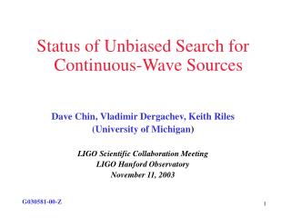
Status of Unbiased Search for Continuous-Wave Sources Dave Chin, Vladimir Dergachev, Keith Riles (University of Michigan ) LIGO Scientific Collaboration Meeting LIGO Hanford Observatory November 11, 2003. G030581-00-Z. Analysis Strategy

E N D
Status of Unbiased Search for Continuous-Wave Sources Dave Chin, Vladimir Dergachev, Keith Riles (University of Michigan) LIGO Scientific Collaboration Meeting LIGO Hanford Observatory November 11, 2003 G030581-00-Z
Analysis Strategy • Measure power in selected bins of averaged periodograms • Bins defined by source parameters (f, RA, d) • Estimate noise level & statistics from neighboring bins • Set “raw” upper limit on quasi-sinusoidal signal on top of empirically determined noise • Scale upper limit by antenna pattern correction, Doppler modulation correction, orientation correction • Refine corrected upper limits further with results from explicit signal simulation
Overview of Data Pipeline for Unbiased All-Sky CW Search Raw Data Simulated Data Create 30-min SFT’s Creation of Power Statistic • Loop over frequency and sky: • Determine search range and control sample range • Determine upper limit on detected power • Apply efficiency corrections (Doppler, AM, orientation • Determine limit on h0 and store Determine efficiency corrections
Creation of Power Statistic and finding upper limits Simulated Data Raw Data 1800-second raw data (Vladimir) Medusa system 1800-second calibrated SFT’s • Power Statistic Creation: (Vladimir) • Simplest: Average calibrated powers bin-by-bin • Allow summation of raw and simulated SFT’s • Apply epoch vetoes (high noise, bad calibration, artifacts) Michigan computers Upper Limits Finder (Vladimir/Dave/Keith)
Upper Limits Finder (schematic) • Loop over values of f0 (SSB frame), RA, sin(δ) in steps of • ¼ (0.5 mHz): • Determine the freq bin(s) of search and the large control range (nearly neighboring) • Compare total power in bin(s) and compare with histogram to find upper limit (~2σ) on detected power in h • Apply efficiency corrections (Doppler modulation, antenna pattern, worst orientation) to find 95% C.L. upper limit on h flux at earth • Store upper limit fDetected Measure Counts Upper limit Power (h2)
SFT Generation Problem: Need 30-minute SFT’s but calibration drifts non-negligible at times. Want a method to use 1-minute calibration α coefficients with minimal new artifacts. • [see talk on Wednesday] • Two frequency-domain calibration procedures tried (“stitched” and “0-order”) • 1) Stitched: (discussed at Hannover meeting) • Create 1-minute SFT’s (high-passed & Tukey-windowed • Apply 1-minute calibration info, window again in Fourier domain • Compute inverse transforms, window again, and stitch to make 30-minute interval • Compute SFT from 30-minute interval • Machinery is in place with flexible control of parameters: • Tukey window ramp intervals • High-pass and low-pass filtering • Strong-line suppression (mean-padding in Fourier domain) • Troubles: Periodic windowing introduces 1/60 Hz residual “comb” • Does not behave correctly in limit of constant calibration
SFT Generation (cont.) • 2) 0-order: • For each 1-minute interval, treat calibration for all bins as the calibration for bin n Apply scale factor to all data based on Rn(t) variation (smoothed) • Fourier transform of bins other than n will be incorrect, but one hopes that bin n correctly accounts for time-varying calibration • But method produces leakage from neighboring bins. Leakage amount depends on discontinuity between start/end points of Rn(t) for 30-minute interval. • Windowing reduces leakage. Overlapped Hann mitigates noise increase. • Behaves correctly in limit of constant calibration • Xavier has also looked at • Averaging of calibration coefficients over 30-minute interval • Direct time-domain calibration via filtering (talk on Wednesday)
SFT Generation (cont.) The unbiased search analysis is relatively robust against the SFT calibration method used – windowing acceptable But we have hoped that our 30-minutes SFT’s would be useful to the rest of the group, i.e., significant SNR is not lost in a coherent search. So how do the methods compare in computing the F statistic? Tried looking at S2 hardware injections (2 pulsars in three IFO’s)
SFT Generation (cont.) Inconclusive – Need more HW injection examples Fortunately, we have 30 to look at in S3 – stay tuned…
Sample Power Statistic density H1 650-670 Hz 11th harmonic of 60 Hz & upconversion visible, but floor is clean • Expect exponential distribution for power in each SFT bin vs time. • Kolmogorov-Smirnov statistic using median to define reference curve
Another H1 band (430-442 Hz) K-S statistic Power density If all bands of all three IFO’s looked this good, then setting limits would be straightforward (away from line artifacts) Unfortunately, reality intrudes…
Average power spectral density in 430-442 Hz band vs time in S2 run – Using last ~1/3 of run
A wide L1 band (200-400 Hz) K-S Count Power density
H1: 0-2000 Hz Mostly okay below 1 kHz • L1: 0-2000 Hz • Mostly badly non-exponential Needs investigation Alternative diagnostic – number of bins in 0.1 Hz bin inconsistent with exponential noise distribution (max=180)
Status and Plans • Have spent much time exploring how to create calibrated 30-minute SFT’s for non-stationary interferometers: • Have a workable solution for our analysis • Not sure yet whether it will work for other pulsar subgroups (other methods under exploration by other group members) • Anxious now to focus on search analysis itself • Now turning more attention to • Efficient search engine construction • Frequency domain artifacts • Handling non-stationarity (veto vs noise-weighting)
Status and Plans (cont.) Can set rough limits now on sources by manually scaling up noise floor by sky-direction-dependent efficiency factors, but have not completed a systematic pipeline to crunch numbers and automatically handle artifacts. Also have not yet tried to exploit multi-IFO analysis to eliminate site-local artifacts, but straightforward baseline approach is to take best limit from the three IFO’s per search point (sky / frequency bin). Plan to have presentable S2 limits by March LSC meeting


![Unbiased All-Sky Search (Michigan) [as of August 17, 2003] [ D. Chin, V. Dergachev, K. Riles ]](https://cdn1.slideserve.com/3372174/unbiased-all-sky-search-michigan-as-of-august-17-2003-d-chin-v-dergachev-k-riles-dt.jpg)