Robot Lab: Robot Path Planning
Robot Lab: Robot Path Planning. William Regli Department of Computer Science (and Departments of ECE and MEM) Drexel University. Introduction to Motion Planning. Applications Overview of the Problem Basics – Planning for Point Robot Visibility Graphs Roadmap Cell Decomposition


Robot Lab: Robot Path Planning
E N D
Presentation Transcript
Robot Lab:Robot Path Planning William RegliDepartment of Computer Science(and Departments of ECE and MEM)Drexel University Slide 1
Introduction to Motion Planning • Applications • Overview of the Problem • Basics – Planning for Point Robot • Visibility Graphs • Roadmap • Cell Decomposition • Potential Field Slide 2
Goals • Compute motion strategies, e.g., • Geometric paths • Time-parameterized trajectories • Sequence of sensor-based motion commands • Achieve high-level goals, e.g., • Go to the door and do not collide with obstacles • Assemble/disassemble the engine • Build a map of the hallway • Find and track the target (an intruder, a missing pet, etc.) Slide 3
Fundamental Question Are two given points connected by a path? Slide 4
Basic Problem • Problem statement: Compute a collision-free path for a rigid or articulated moving object among static obstacles. • Input • Geometry of a moving object (a robot, a digital actor, or a molecule) and obstacles • How does the robot move? • Kinematics of the robot (degrees of freedom) • Initial and goal robot configurations (positions & orientations) • Output Continuous sequence of collision-free robot configurations connecting the initial and goal configurations Slide 5
Example: Rigid Objects Slide 6
Example: Articulated Robot Slide 7
Is it easy? Slide 8
Hardness Results • Several variants of the path planning problem have been proven to be PSPACE-hard. • A complete algorithm may take exponential time. • A complete algorithm finds a path if one exists and reports no path exists otherwise. • Examples • Planar linkages [Hopcroft et al., 1984] • Multiple rectangles [Hopcroft et al., 1984] Slide 9
Tool: Configuration Space Difficulty • Number of degrees of freedom (dimension of configuration space) • Geometric complexity Slide 10
Extensions of the Basic Problem • More complex robots • Multiple robots • Movable objects • Nonholonomic & dynamic constraints • Physical models and deformable objects • Sensorless motions (exploiting task mechanics) • Uncertainty in control Slide 11
Extensions of the Basic Problem • More complex environments • Moving obstacles • Uncertainty in sensing • More complex objectives • Optimal motion planning • Integration of planning and control • Assembly planning • Sensing the environment • Model building • Target finding, tracking Slide 12
Practical Algorithms • A complete motion planner always returns a solution when one exists and indicates that no such solution exists otherwise. • Most motion planning problems are hard, meaning that complete planners take exponential time in the number of degrees of freedom, moving objects, etc. Slide 13
Practical Algorithms • Theoretical algorithms strive for completeness and low worst-case complexity • Difficult to implement • Not robust • Heuristic algorithms strive for efficiency in commonly encountered situations. • No performance guarantee • Practical algorithms with performance guarantees • Weaker forms of completeness • Simplifying assumptions on the space: “exponential time” algorithms that work in practice Slide 14
Problem Formulation for Point Robot • Input • Robot represented as a point in the plane • Obstacles represented as polygons • Initial and goal positions • Output • A collision-free path between the initial and goal positions Slide 15
Framework Slide 16
Visibility Graph Method • Observation: If there is a collision-free path between two points, then there is a polygonal path that bends only at the obstacles vertices. • Why? • Any collision-free path can be transformed into a polygonal path that bends only at the obstacle vertices. • A polygonal path is a piecewise linear curve. Slide 17
Visibility Graph • A visibility graphis a graph such that • Nodes: qinit, qgoal, or an obstacle vertex. • Edges: An edge exists between nodes u and v if the line segment between u and v is an obstacle edge or it does not intersect the obstacles. Slide 18
Computational Efficiency • Simple algorithm O(n3) time • More efficient algorithms • Rotational sweep O(n2log n) time • Optimal algorithm O(n2) time • Output sensitive algorithms • O(n2) space Slide 20
Framework Slide 21
Breadth-First Search Slide 22
Breadth-First Search Slide 23
Breadth-First Search Slide 24
Breadth-First Search Slide 25
Breadth-First Search Slide 26
Breadth-First Search Slide 27
Breadth-First Search Slide 28
Breadth-First Search Slide 29
Breadth-First Search Slide 30
Breadth-First Search Slide 31
Other Search Algorithms • Depth-First Search • Best-First Search, A* Slide 32
Framework Slide 33
Summary • Discretize the space by constructing visibility graph • Search the visibility graph with breadth-first search Q: How to perform the intersection test? Slide 34
Summary • Represent the connectivity of the configuration space in the visibility graph • Running time O(n3) • Compute the visibility graph • Search the graph • An optimal O(n2) time algorithm exists. • Space O(n2) Can we do better? Slide 35
Classic Path Planning Approaches • Roadmap – Represent the connectivity of the free space by a network of 1-D curves • Cell decomposition – Decompose the free space into simple cells and represent the connectivity of the free space by the adjacency graph of these cells • Potential field – Define a potential function over the free space that has a global minimum at the goal and follow the steepest descent of the potential function Slide 36
Classic Path Planning Approaches • Roadmap– Represent the connectivity of the free space by a network of 1-D curves • Cell decomposition – Decompose the free space into simple cells and represent the connectivity of the free space by the adjacency graph of these cells • Potential field – Define a potential function over the free space that has a global minimum at the goal and follow the steepest descent of the potential function Slide 37
Roadmap • Visibility graph Shakey Project, SRI [Nilsson, 1969] • Voronoi Diagram Introduced by computational geometry researchers. Generate paths that maximizes clearance. Applicable mostly to 2-D configuration spaces. Slide 38
Voronoi Diagram • Space O(n) • Run time O(n log n) Slide 39
Other Roadmap Methods • Silhouette First complete general method that applies to spaces of any dimensions and is singly exponential in the number of dimensions [Canny 1987] • Probabilistic roadmaps Slide 40
Classic Path Planning Approaches • Roadmap – Represent the connectivity of the free space by a network of 1-D curves • Cell decomposition – Decompose the free space into simple cells and represent the connectivity of the free space by the adjacency graph of these cells • Potential field – Define a potential function over the free space that has a global minimum at the goal and follow the steepest descent of the potential function Slide 41
Cell-decomposition Methods • Exact cell decomposition The free space F is represented by a collection of non-overlapping simple cells whose union is exactly F • Examples of cells: trapezoids, triangles Slide 42
Trapezoidal Decomposition Slide 43
Computational Efficiency • Running time O(n log n) by planar sweep • Space O(n) • Mostly for 2-D configuration spaces Slide 44
Adjacency Graph • Nodes: cells • Edges: There is an edge between every pair of nodes whose corresponding cells are adjacent. Slide 45
Summary • Discretize the space by constructing an adjacency graph of the cells • Search the adjacency graph Slide 46
Cell-decomposition Methods • Exact cell decomposition • Approximate cell decomposition • F is represented by a collection of non-overlapping cells whose union is contained in F. • Cells usually have simple, regular shapes, e.g., rectangles, squares. • Facilitate hierarchical space decomposition Slide 47
Quadtree Decomposition Slide 48
Octree Decomposition Slide 49
Algorithm Outline Slide 50