Download
1 / 17
170 likes | 293 Vues
This chapter delves into the thermodynamic properties associated with the mixing of components in solutions and mixtures. It explores concepts such as the entropy of mixing, energy of mixing, and free energy changes when two substances are combined. Using the lattice model, it outlines equations for calculating mixing entropy (∆Smix), internal energy (∆Umix), and free energy (∆Fmix). The section also covers essential parameters such as the exchange parameter (χAB) and the implications of ideal versus non-ideal solutions.

E N D
Solutions and Mixtures Chapter 15 # Components > 1 Lattice Model Thermody. Properties of Mixing (S,U,F,)
I. Entropy of Mixing • Translational Entropy of Mixing • Assume N lattice sites filled completely with NA A molecules and NB B molecules so that N = NA + NB. • Then W = N!/( NA! NB!) See Ch 6 • Smix = k ℓn W = - k(NAℓn xA + NBℓn xB) = -Nk (xAℓn xA + xBℓn xB) Eqn 15.2, 3 • Ex 15.1
II. Energy of Mixing (1) • Assume ideal soln, then, Umix= 0 and Fmix= -TSmix • If the soln is not ideal, then Umix = sum of contact interactions of noncovalent bonds of nearest neighbor pairs 0. • U = mAA wAA + mAB wAB + mBB wBB where mIJ = # I-J bonds and wIJ = I-J contact energies. All w terms < 0
Energy of Mixing (2) • Define mAA and mAB = f(mAB, NA, NB) • Each lattice site has z sides, so z NA = total number of contacts for all A • Then zNA = 2mAA + mAB. And zNB = 2mBB + mAB . Solve for mAA and mBB • Use to find U = (zwAA)NA/2 + (zwBB)NB/2 + ([wAB- ½ (wAA + wBB)] mAB) Eqn 15.8
Energy of Mixing (3) • To simplify Eqn 15.8, use the Bragg-Williams or mean-field approximation to find average <mAB>. Note that this is a simplification and we assume that this average is a good approx to the actual situation. (i.e. one distribution dominates vs using a distribution of mAB values.
Energy of Mixing (4)Mean-Field Approximation • Assume A and B are mixed randomly. Then the probability of finding a B next to an A ≈ z x(1-x) where pA = x = xA and (1-x) = pB. • Then mAB = z Nx(1-x). Plug into Eqn 15.8 for U to get final eqn for U = Eqn 15.10. • U = (zwAA)NA/2 + (zwBB)NB/2 + kT ABNANB/N
Energy of Mixing (5)Exchange Parameter • U = (zwAA)NA/2 + (zwBB)NB/2 + kT ABNANB/N • AB = energy cost of replacing A in pure A with B; similarly for B. • AB = exchange parameter = - ℓn Kexch • Umix = RT ABxA xB
Energy of Mixing (6)Exchange Parameter • AB = exchange parameter = - ℓn Kexch • A + B ↔ mixing eq. constant Kexch • Umix = RT ABxA xB • AB can be > 0 (AB interactions weaker than AA and BB); little mixing and Umix more positive, Kexch smaller • AB can be < 0 (AB stronger than AA and BB), …
III. Free Energy of Mixing (1) • F = U – TS = [Eqn 15.11] – T [Eqn 15.2] = Eqn 15.12 • Pure A + pure B mixed A + B has Fmix = F(NA + NB) – F(NA, 0) – F(0,NB) • Note that F(NA, 0) = ½ x wAANA • Fmix= [x ln x + (1-x) ln(1-x) + AB x(1-x)]NkT Eqn 15.14 • This eqn describes a regular solution.
Free Energy of Mixing (2) • If Fmix > 0, minimal mixing to form a soln. • If Fmix < 0, then a soln forms • If soln separates into 2 phases, Eqn 15.14 does not apply. • Ex 15.2
IV. Chemical Potentials and Mixing • A = (F/NA)NB,T = kT ℓn xA + zwAA/2 + kTAB (1-xA)2 = kT ℓn xA + corections due to AA interactions and exchange parameter. Eqn 15.15 • Also = 0 + kT ℓn x where = activity coefficient. x = effective mol fraction.
V. Free Energy of Creating Surface Area • Consider interface or boundary between 2 condensed phases A and B. • AB = interfacial tension = free energy cost of increasing the interfacial area between A and B. • Calculate AB using the lattice model.
Surface Area (2) • Assume (Fig 15.7) • A and B are the same size • NA = # A molecules and NB = B molecules • interface consists of n A and n B molecules in contact with each other • bulk molecules have z A nearest neighbors • surface A molecules have (z-1) A nearest neighbors
Surface Area (3) • U = Σ ni wij = term for A in bulk + term for A at surface + term for AB interactions + term for B in bulk + term for B at surface • Then U = Eqn 15.19 = F since S = 0 • Let A = total area of interface = na • Let a = area per molecule exposed to surface • Then AB = (F/A)NB,NA,T = (F/n) (n/A) AB = [wAB – ½ (wAA + wBB)]/a
Surface Area (4) • Then AB = (F/A)NB,NA,T = (F/n) (n/A) = [wAB – ½ (wAA + wBB)]/a • AB = (kT/za) AB Eqn 15.22; see Eqn 15.11 • If there are no B molecules Eqn 15.22 reduces to Eqn 14.28 AB = - wAA /2a • Ex 15.3 (mixing is not favorable, see p. 273)
Surface Area (5) • Assumptions • Mean field approximation for distribution • Only translational contributions to S, U, F and μ are included. • What about rot, vib, electronic? We assume that in mixing, only translational (location) and intermolecular interactions change. • Then Fmix = F(NA + NB) – F(NA, 0) – F(0,NB) = NkT[x ln x + (1-x) ln (1-x) + AB x(1-x)]
Surface Area (6) • However, if chemical rxns occur, rot, vib and elec must be included.