Download
1 / 21
210 likes | 357 Vues
Secular variation in Germany from repeat station data and a recent global field model Monika Korte and Vincent Lesur Helmholtz Centre Potsdam, German Research Centre for Geosciences - GFZ. Outline: Motivation German repeat station data The global field model GRIMM-2

E N D
Secular variation in Germany from repeat station data and a recent global field modelMonika Korte and Vincent LesurHelmholtz Centre Potsdam, German Research Centre for Geosciences - GFZ Outline: • Motivation • German repeat station data • The global field model GRIMM-2 • Comparison of secular variation of model and data • Conclusions
Motivation • Since 1999 satellites like Ørsted and CHAMP provide a dense global geomagnetic data coverage. • These, together with geomagnetic observatory data, lead to increa-singly accurate global field models with good secular variation descriptions. • Do repeat station data from areas with relatively good observatory coverage provide additional useful signal?
German repeat station data - Overview • Repeat station measurements in Germany started in 1999/2000 • Improved data processing with local/regional variometer • 12 variometer stations used in nearly each survey • 3 geomagnetic observatories (WNG, NGK, FUR – BFO only established in 2005)
Why local variometers? Data processing to obtain internal field annual means for repeat stations: C(xi,tmean) = C(xi,ti) – C(O,ti) + C(O, tmean) Repeat station“annual mean”of component C Repeat stationmeasurementvalue at time ti Observatoryannual meanof component C Observatoryrecording attime ti This difference can be determined more robustlyfrom (quiet) night time differences with a local variometer Assumptions: - Secular variation is the same - External variations are the same - Induced variations are the same at repeat station and observatory
German repeat station data - Details • Surveys in 1999/2000 (half network per year)2001/2002 (half network per year)2003 (about 75% of full network)2004 (full network)2006 (full network) 2008 (full network) • All data reduced to annual mean centered on the middle of the year the measurements were done.
Global field model GRIMM2 • Continuous model valid for 2001 – 2008
Global field model GRIMM2 - Data • CHAMP satellite data- X and Y in solar-magnetic (SM) coordinates between +/-55° magnetic latitude- geocentric X,Y,Z at high latitudes - selected for quality: acceptabel quality flags, corrected for orientation errors- selected for magnetically quiet data: IMF Z-componente positive, Vector Magnetic Disturbance (Thomson & Lesur, 2007) < 20 nT and norm of its derivative < 100 nT/day - low/mid latitude data addionally selected by local time: LT between 23:00 and 5:00, sun below horizon • Observatory data- hourly means in same coordinate systems and with same selection criteria applied
Global field model GRIMM2 - Modelling • Core field and secular variation- spherical harmonics with time dependence by 5th order B-splines up to SH degree 16, knot-point spacing 400days- weak regularization by minimizing squared second time derivative of radial field at the CMB (high degree core field SH degrees influenced)- additional regularization to mitigate effect of additional degrees of freedom introduced by 5th order B-splines: minimizing squared third time derivative of radial field at Earth’s surface (low SH degrees influenced) • Toroidal magnetic field modelled to take into account field aligned currents over polar regions (constant term with annual variation) • Ionospheric field over polar regions modelled by assumption of temporally varying currents in a thin shell (110 km above Earth)
Comparison of global model and annual means data • “Annual means” of GRIMM2 obtained as average of 10 core field values per year • Model values subtracted fromrepeat station and observatoryannual means • Annual mean data are notfree from external fieldvariations!(Example: annual means of European observatories orderedby geomag. Latitude with CM4 model core field subtracted)
Empirical external field correction WNG NGK FUR 1. Core fieldmodel removed:- lithospheric offset - external field influences 2. Constant offsetsremoved: - homogeneousresidual patternBlack lines:average resisualpattern 3. Average residual patternremoved fromdata (black lines)
Field change from 2000.5 to 2008.5 Rather linear change X: ca. 70 nT or 9nT/yr Y: ca. 300 nT or 38 nT/yr Z: ca. 250 nT or 31 nT/yr NGK annual means
Locations of repeat stations withlocal variometer Vertical component Z North component X East component Y Vector anomaly mapsR-SCHA model by Korte & Thébault, 2007
Scatter or systematic trends? • Measurement uncertainties from scatter among measurements at one location in the order of D (Y) 1.6 nT H (X) 1 nT Z 0.7 nT • Linear regression of variometer station time series:- trend up to +/- 1.1 nT/yr occur in all components- trends mostly in the order of 0 to 0.5 nT/yr in all components- often low correlation • Problem: global model not reliable for 2000.5 and 2008.5 (ends),linear regression of data between 2001.5 and 2006.5 only (3 to 4 epochs per time series only, no proper statistics!):- trends in the same order in general, but hardly similar at the same stations- low correlation for about half of the time series
Scatter or systematic trends? • Results where similar linear trends exist and correlation is [high:- tel X (0.53 nT/yr), Y (-0.51 nT/yr), Z (-0.56 nT/yr)- eil Y (-0.99 nT/yr)- [kar X (-0.53 to -0.63 nT/yr)] • These values are rather high, but not completely unreasonable compared to theory:Thébault et al. (2009) investigated the expected induced signal based on the vertically integrated susceptibility (VIS) model by Hemant and Maus (2005). Their results are:* 0.1 nT/yr for western Europe* up to 0.3 – 0.6 nT/yr for eastern Europe* maximal globally (very few regions) 0.65 – 1.3 nT/yr
Tentative interpolation of linear trends in residuals Vertical component Z North component X East component Y
Anomalies and linear trend - X North component X North component X
Anomalies and linear trend - Y East component Y East component Y
Anomalies and linear trend - Z Vertical component Z Vertical component Z
Residuals of further repeat stations Scatter of up to 10 nT in time series at many locationswithout variometer
Conclusions • Regional secular variation is described well by recent global field models based on satellite and observatory data. • High accuracy repeat station data might provide information about induced sources of crustal field, but it is very difficult to discriminate between signal and noise • Longer time series are needed for more reliable statistics